Understanding Stochastic Gradient Descent in Machine Learning: A Beginner’s Guide

Stochastic Gradient Descent (SGD) is a core technique for training machine learning models. Machine learning is all about finding the best parameters that minimize errors on data. But with countless possibilities, how do algorithms pick the right ones? That’s where optimization methods like SGD come in.

Instead of scanning entire datasets at once, SGD updates parameters step-by-step using small data batches. This makes it faster and more practical, especially for large datasets, helping machine learning models learn without slowing down or getting overwhelmed.

But what is SGD, and why is it needed to optimize datasets in machine learning? This blog will discuss SGD variants, along with their advantages and challenges compared to Gradient Descent in machine learning. 

Struggling to make sense of large datasets or optimize your ML models efficiently? Gain practical skills in algorithms like SGD and more through structured learning and mentorship from industry experts. Explore the Artificial Intelligence & Machine Learning courses from upGrad and take the next step in your ML journey.

What is Stochastic Gradient Descent? Definition and Importance

Stochastic Gradient Descent (SGD) is an optimization algorithm used to train machine learning models by minimizing the loss function, i.e., the gap between predicted and actual outcomes. It's a more agile version of the traditional Gradient Descent algorithm, designed to handle large datasets efficiently and adapt to situations where parameters can take on negative values.

Classic Gradient Descent updates parameters after scanning the entire dataset, which is accurate but slow and resource-heavy. SGD speeds things up by updating after each data point or mini-batch, making it ideal for large datasets, real-time tasks, and online learning, where models learn continuously from streaming or real-time data.

Want to build models that can handle large-scale data without slowing down? Learn how to apply faster, scalable techniques like SGD with real-world projects and industry mentorship. Here are the top 3 courses that align best with the need for practical, scalable machine learning training:

• Executive Diploma in Machine Learning and AI with IIIT-B
• Masters in Artificial Intelligence and Machine Learning - IIITB Program
• Advanced Generative AI Certification Course

Difference Between Stochastic Gradient Descent & Gradient Descent in ML

Let’s look at the key differences between Gradient Descent and Stochastic Gradient Descent in machine learning:

In short, SGD strikes a balance between speed and accuracy, allowing models to learn efficiently even when the dataset size becomes a challenge. 

Also Read: Understanding Gradient Descent in Logistic Regression: Guide for Beginners

Now, let’s understand the working of the Stochastic Gradient Descent algorithm in Machine Learning. 

How SGD Works in Machine Learning

Imagine you are blindfolded and trying to find the lowest point in a valley. In Gradient Descent (GD), you would measure the slope of the entire valley before taking a step, ensuring you move in the right direction. While this method is accurate, it’s slow, especially when the valley (or dataset) is large.

On the other hand, Stochastic Gradient Descent (SGD) takes a more immediate approach. It measures the slope at a single spot and adjusts the direction right away, even if that direction isn’t perfect. While this introduces some randomness, it allows SGD to take faster steps, adjust parameters more frequently, and quickly head toward the bottom of the valley.

Mathematically:

Gradient Descent (GD) updates parameters using the entire dataset:

Where:

• 𝜂 is the learning rate, controlling the step size.
• ∇ 𝜃J(θ) is the gradient of the cost function, calculated over the whole dataset.

This method ensures accurate updates but at a high computational cost, especially for large datasets, while using batch gradient in ML.

Stochastic Gradient Descent (SGD), however, updates parameters using only a single data point at a time:

Here:

• 𝑥 (i)  and 𝑦 (i)  represent the features and target value for a single data point.
• The gradient is calculated based on just that single sample.

This introduces some noise in the updates, but the advantage is clear: by processing one data point (or a small batch) at a time, the algorithm can update much more frequently, speeding up the learning process.

Ready to take your machine learning skills further and explore the latest advancements in AI? upGrad’s Generative AI Mastery Certificate for Software Development, offered in partnership with Microsoft, provides hands-on training to build and deploy generative models. 

Now that you understand the working of SGD in machine learning better, let’s look at its variants. 

Exploring the 6 Variants of Stochastic Gradient Descent in Machine Learning

Stochastic Gradient Descent (SGD) is a flexible algorithm, with its variants providing solutions to particular challenges such as speed, convergence stability, and accommodating various types of data. Let’s explore six common variants and their use cases.

1. Mini-batch SGD

Mini-batch SGD splits the dataset into small batches (e.g., 32 or 64 data points) rather than using a single data point or the entire dataset for each update. This strikes a balance between the slow but accurate updates of full-batch Gradient Descent (GD) and the noisy, faster updates of plain SGD. The batch size is important to tune, as smaller batches introduce more noise but can help escape local minima, while larger batches produce smoother updates closer to full-batch GD.

• Use Case:

Mini-batch SGD is widely used in deep learning, particularly in training neural networks. By processing small batches, it makes use of the parallelization capabilities of modern hardware (like GPUs), speeding up training without losing too much accuracy. It’s especially effective when working with large datasets, as it strikes a balance between computation efficiency and model convergence.

• Example:

In image classification with convolutional neural networks (CNNs), mini-batch SGD processes batches of images (e.g., 32 or 64) to update the network’s weights. The choice of batch size can significantly affect the training speed and final performance.

Also Read: Categories of Machine Learning: What Classes of Problems Do They Solve?

2. Momentum

Momentum introduces a velocity term to the update rule, which considers past gradients along with the current gradient in ML to determine the direction of the update. This helps the model avoid oscillations and provides a smoother, faster convergence, especially in regions with steep or flat gradients. The momentum effect is controlled by a hyperparameter, typically set around 0.9, that balances how much past gradients influence the current update.

• Use Case:

Momentum is useful in cases where the cost function has areas of steep descent or flat regions, as it helps the algorithm gain speed when moving down slopes and prevents it from oscillating around the minima.

• Example:

Imagine training a model on a dataset with sharp, jagged valleys (steep gradients) and flat plateaus. Momentum allows the model to keep moving quickly through the steep regions and smooth out its path when it hits a flat region, ensuring faster convergence to the optimal solution.

Also Read: Big Data Tutorial for Beginners: All You Need to Know

3. Nesterov Accelerated Gradient (NAG)

Nesterov Accelerated Gradient is an enhanced version of momentum. It anticipates the next step by looking ahead at the velocity before updating the parameters. This extra "look ahead" improves the convergence speed, making NAG more efficient than standard momentum, especially in regions with flat gradients.

• Use Case:

NAG is commonly used in complex optimization tasks like training deep neural networks, where the model's performance heavily depends on fast, smooth convergence.

• Example:

In training a deep neural network for image recognition, NAG helps the model adjust weights more effectively by making a parameter update based not just on the current gradient but also on the momentum of previous gradients, optimizing performance.

Also Read: Data Preprocessing in Machine Learning: 7 Key Steps to Follow, Strategies, & Applications

4. Adagrad

Adagrad (Adaptive Gradient Algorithm) adapts the learning rate for each parameter individually. It adjusts the learning rate based on the past gradients, making it particularly effective for dealing with sparse data. Parameters with large gradients see their learning rates reduced, while those with smaller gradients get increased rates. However, a major limitation of Adagrad is that its learning rates shrink continuously over time, which can slow down training or even stop learning altogether in later stages.

• Use Case:

Adagrad is especially useful for tasks where the data is sparse, such as natural language processing (NLP), where certain features may appear infrequently but are still crucial for the model.

• Example:

In text classification tasks like spam detection, Adagrad adjusts the learning rates for different words in the text. Rare words, which might be critical for classification but do not appear often, receive larger updates, ensuring they have enough weight in the model.

Also Read: What Is Pattern Recognition and Machine Learning? Importance and Applications

5. RMSProp

RMSProp (Root Mean Square Propagation) modifies Adagrad by using a moving average of squared gradients to prevent rapid shrinking of learning rates. It incorporates a decay term, typically around 0.9, that weights past gradients, allowing the algorithm to maintain a balanced, adaptive learning rate throughout training. This helps avoid the learning rate decay issues that Adagrad can face over time.

• Use Case:

RMSProp is commonly used in training recurrent neural networks (RNNs) and other deep learning models that require adaptive learning rates over time.

• Example:

When training an RNN for language translation, RMSProp helps the model maintain an optimal learning rate, especially when dealing with long data sequences. The moving average of squared gradients ensures that the learning rate doesn’t become too small and stall learning.

Also Read: Recurrent Neural Network in Python: Ultimate Guide for Beginners

6. Adam (Adaptive Moment Estimation)

Adam combines the ideas of momentum and RMSProp. It calculates adaptive learning rates for each parameter by using both the first moment (mean) and second moment (variance) of the gradients. This makes Adam an effective optimizer that requires less manual tuning and adapts well to a wide variety of problems.

• Use Case:

Adam is one of the most popular optimizers for deep learning tasks. It’s widely used in models like deep neural networks, where it often outperforms other optimization methods in terms of training speed and convergence.

• Example:

In training a complex neural network for image classification, Adam adapts the learning rates dynamically for each weight based on both the momentum (past gradients) and the magnitude of the gradients. This helps the model converge quickly, even in large-scale problems like training on datasets such as ImageNet.

Also Read: Image Segmentation Techniques [Step By Step Implementation]

When to Use Which SGD Variant?

Each of these variants helps overcome specific challenges faced during model training. Choosing the right variant depends on the problem at hand and the particular needs of the dataset or model you’re working with. Here’s what to consider when selecting an SGD variant for your dataset. 

Also Read: What is Machine Learning and Why it matters

Once you have selected the required variant as per your problem, it's time to implement the Stochastic Gradient Descent algorithm in machine learning. 

Step-by-Step Guide for Implementing SGD in Machine Learning

Let's go through the entire process of implementing a simple univariate linear regression model using Stochastic Gradient Descent (SGD) in Python. At each step, we’ll elaborate on the logic behind the code and what happens in the process.

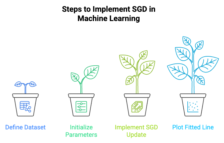
Step 1: Define the Dataset

In this step, we generate the dataset. We define the feature X (input) and target y (output), where y follows a linear relationship with X but includes some noise for realism.

import numpy as np
import matplotlib.pyplot as plt

# Sample data: y = 2x + 1 with some noise
X = np.linspace(0, 10, 100)
y = 2 * X + 1 + np.random.randn(100) * 1.5

Explanation:

• We are creating a dataset where the true relationship between X (the input) and y (the target) follows the equation 𝑦 = 2𝑥 + 1. To make it more realistic, we add some noise to the target variable y using np.random.randn(100) * 1.5. This makes the data more challenging and similar to real-world data, which often has noise.
• X = np.linspace(0, 10, 100) generates 100 evenly spaced values between 0 and 10 to simulate the feature variable.
• The noise term np.random.randn(100) * 1.5 generates random noise, making the target values y deviate from the perfect linear equation.

Step 2: Initialize Parameters

Here, we initialize the model's parameters. We start with zero values for the intercept (theta_0) and slope (theta_1). We also define the learning rate and number of epochs for training.

theta_0 = 0  # intercept
theta_1 = 0  # slope
learning_rate = 0.01
epochs = 50

Explanation:

• theta_0 and theta_1 are the initial values for the intercept and slope of our linear regression model. These parameters will be updated during the training process using SGD.
• learning_rate = 0.01 defines the step size for each update. A smaller learning rate means smaller steps, leading to more gradual learning but potentially slower convergence.
• epochs = 50 defines how many times we will iterate through the entire dataset. In SGD, each epoch means we process all data points once, but the parameters are updated after each data point.

Step 3: Implement SGD Update

In this step, we implement the Stochastic Gradient Descent algorithm. We update the model parameters (theta_0 and theta_1) after each data point by calculating the gradients and adjusting the parameters accordingly.

n = len(X)
for epoch in range(epochs):
    for i in range(n):
        y_pred = theta_0 + theta_1 * X[i]
        error = y_pred - y[i]
        
        # Gradients
        grad_0 = error
        grad_1 = error * X[i]
        
        # Update parameters
        theta_0 = theta_0 - learning_rate * grad_0
        theta_1 = theta_1 - learning_rate * grad_1

Explanation:

• We loop through the dataset multiple times (for epochs), and within each epoch, we process each data point one by one.
• Prediction (y_pred): The model predicts the value of y for the given X[i] using the current parameters theta_0 (intercept) and theta_1 (slope).
• Error Calculation: The error is the difference between the predicted value (y_pred) and the actual target value (y[i]). The model is trying to minimize this error during the training process.

Gradient Calculation:

• grad_0 = error: This is the gradient with respect to the intercept. It tells us how much the intercept needs to change in order to reduce the error.
• grad_1 = error * X[i]: This is the gradient with respect to the slope. It tells us how much the slope should change based on the data point X[i] and the error.

Parameter Update:

• theta_0 = theta_0 - learning_rate * grad_0: This updates the intercept by moving it in the direction opposite to the gradient, scaled by the learning rate.
• theta_1 = theta_1 - learning_rate * grad_1: Similarly, this updates the slope.

These updates happen after processing each data point, meaning the parameters are adjusted frequently, which is why SGD is faster compared to traditional gradient descent (which uses the entire dataset).

Step 4: Plot the Fitted Line

Finally, we plot the original data points and the learned regression line. This helps us visualize how well our model fits the data.

plt.scatter(X, y, label='Data Points')
plt.plot(X, theta_0 + theta_1 * X, color='red', label='Fitted Line')
plt.legend()
plt.show()

Explanation:

• The plt.scatter(X, y) function plots the original data points (X and y) as a scatter plot. These points are the noisy data we want to fit the model to.
• plt.plot(X, theta_0 + theta_1 * X, color='red') plots the fitted line, using the learned parameters theta_0 and theta_1. The line represents the model’s best guess for the underlying relationship between X and y.
• Finally, plt.legend() adds a legend to the plot, and plt.show() displays the graph.

Final Output 

Final Output Explanation

After running the above code, you will see a scatter plot with the original noisy data points and a red line representing the linear regression model learned by SGD. The fitted line should approximate the underlying relationship y = 2x + 1, though variation from noise and SGD’s stochasticity will remain. 

Also Read: Linear Regression in Machine Learning: Everything You Need to Know

By now, you must have a better idea of why you should use SGD over Gradient Descent in ML. Let’s look at the advantages and disadvantages of using SGD. 

Pros & Cons of Using Stochastic Gradient Descent in Machine Learning

Stochastic Gradient Descent (SGD) is fast and memory-efficient, making it ideal for large datasets and real-time applications. However, its noisy updates can cause fluctuations in convergence, requiring more epochs and careful tuning of the learning rate for stability. 

Here’s a detailed comparison of its advantages and disadvantages. 

Also Read: Different Types of Regression Models You Need to Know

Now that you have a fair idea of how SGD can be beneficial for your machine learning models, let’s look at its real-time application. 

Application of SGD in Machine Learning

Stochastic Gradient Descent is widely used across various machine learning and deep learning tasks, enabling fast training on large datasets and complex models. Below are key applications of SGD with examples:

1. Deep Learning and Image Classification

SGD, often with mini-batches, powers the training of neural network models on large datasets like ImageNet. It updates model parameters frequently without processing the entire dataset at once, balancing speed and accuracy. Variants like Momentum or Adam help handle noisy gradients and speed convergence.

• Training neural networks for image classification involves using mini-batch SGD, which updates weights incrementally to enhance speed and reduce overfitting.
• Efficiently training Convolutional Neural Networks (CNNs) requires recognizing patterns like edges or faces efficiently using SGD with momentum or adaptive optimizers.

2. Natural Language Processing (NLP)

SGD is ideal for training models on massive text corpora by processing small batches or individual samples.

• Training Word2Vec models involves SGD updating parameters after each word to learn word relationships based on context.
• Another example is training recurrent neural networks (RNNs) for applications such as text classification or machine translation.

Want to deepen your understanding of how algorithms like SGD power machine learning applications such as text analysis? Explore upGrad’s Introduction to Natural Language Processing course to build practical skills and see these concepts in action. Start learning today at no cost and strengthen your AI toolkit.

3. Recommendation Systems

SGD optimizes matrix factorization models that predict user preferences by iteratively updating user and item feature matrices.

• For instance, Netflix’s recommendation engine uses SGD to adjust latent features of users and movies, predicting what content users might enjoy based on their history.

Also Read: Data Modeling for Real-Time Data in 2025: A Complete Guide

Now that you’ve seen how SGD powers a wide range of machine learning applications, it’s time to test your understanding. Take a quick quiz to reinforce what you've learned.

Test Your Knowledge of Stochastic Gradient Descent in Machine Learning

Here’s a quiz to test your understanding of SGD and see how well you grasp its key concepts and applications in machine learning.

1. What is the main difference between Gradient Descent and Stochastic Gradient Descent?

a) Gradient Descent updates parameters after each data point; SGD after the entire dataset

b) Gradient Descent updates parameters after the entire dataset; SGD after each data point or mini-batch

c) Gradient Descent uses mini-batches; SGD uses full batches

d) Gradient Descent and SGD update parameters the same way

2. Why is SGD preferred for large datasets?

a) It processes the entire dataset at once

b) It updates parameters after each small data sample or batch, speeding up training

c) It ignores parts of the dataset

d) It uses more memory than Gradient Descent

3. What role does the learning rate play in SGD?

a) It controls the size of parameter updates during training

b) It determines the number of training epochs

c) It decides the batch size

d) It is irrelevant to parameter updates

4. What is Mini-batch SGD?

a) Using a single data point for each parameter update

b) Using the entire dataset for each parameter update

c) Splitting the dataset into small batches (e.g., 32 or 64 samples) and updating parameters after each batch

d) Ignoring batches and updating randomly

5. How does Momentum improve SGD?

a) It speeds up convergence by averaging past gradients with current ones to smooth updates

b) It slows down training to increase accuracy

c) It randomly changes learning rates

d) It prevents parameter updates altogether

6. What problem can Adagrad solve in SGD?

a) It prevents overfitting by reducing model complexity

b) It adapts learning rates for each parameter individually, helping with sparse data

c) It increases learning rates uniformly

d) It fixes batch size automatically

7. Why might SGD take longer to converge compared to Gradient Descent?

a) Because SGD updates are noisy and based on small samples, causing more fluctuation

b) Because it processes the whole dataset every time

c) Because it uses fixed learning rates only

d) Because it doesn’t update parameters regularly

8. How does Adam combine ideas from other SGD variants?

a) By using momentum and adaptive learning rates together

b) By ignoring gradients altogether

c) By using batch sizes of one only

d) By fixing learning rates throughout training

9. Can SGD escape local minima better than GD? Why?

a) No, both behave the same

b) Yes, because the noisy updates in SGD can help jump out of local minima

c) No, SGD gets stuck faster

d) Yes, because SGD processes the entire dataset each time

10. In what kinds of machine learning tasks is SGD most commonly applied?

a) Only small datasets with few features

b) Large-scale tasks like deep learning, NLP, image classification, and recommendation systems

c) Tasks that don’t require training

d) Only for unsupervised learning

If you're looking to strengthen your foundation in machine learning, start with upGrad's Basic Python Programming course. It’s designed for beginners and covers essential Python concepts crucial for data science and machine learning. Learn at your own pace with hands-on projects and expert guidance to kickstart your journey in tech.

Learn Stochastic Gradient Descent in Machine Learning with upGrad

SGD efficiently trains machine learning models by updating parameters in small data batches, balancing speed and accuracy. Variants like Mini-batch SGD, Momentum, and Adam enhance stability and convergence. It's crucial to have a strong programming foundation to effectively understand and apply stochastic gradient descent (SGD). 

upGrad offers beginner-friendly courses like the Basic Python Programming course, which is a great starting point for those new to coding. The course covers essential Python concepts, such as data types, functions, and loops, which are the building blocks for implementing machine learning algorithms like SGD.

Once you're comfortable with Python, you can expand your skills further with more specialized courses such as:

• Executive Post Graduate Certificate Programme in Data Science & AI
• Master’s Degree in Artificial Intelligence and Data Science
• Professional Certificate Program in Data Science and AI

Feeling uncertain about the right career path or the skills you need to succeed? Reach out to upGrad’s expert counselors who can help you identify the best course based on your goals and current skill set. Whether online or at our offline centers, we’re here to help you take the next step forward.

FAQs

1. What is the main difference between Gradient Descent and Stochastic Gradient Descent?

Traditional Gradient Descent computes the gradient using the entire dataset before performing a parameter update. This method provides a stable and smooth convergence path but becomes computationally intensive for large datasets. On the other hand, Stochastic Gradient Descent (SGD) updates the parameters after evaluating each individual data point. While this introduces more fluctuation in the updates, it significantly speeds up training and can help the model escape local minima by exploring the solution space more dynamically.

2. Why is SGD preferred for large datasets?

SGD processes data points individually or in small batches, avoiding the need to load the entire dataset into memory. This makes it highly efficient and scalable for large datasets where full-batch methods would be impractical. By performing frequent updates, it allows models to start learning and improving early in the training process. It also aligns well with online learning and streaming data environments where data arrives continuously.

3. What impact does the learning rate have on SGD’s training process?

The learning rate controls how much the model's parameters change during each update. A large learning rate can lead to rapid learning but risks instability, where the model overshoots the optimal values. A small learning rate provides more precise convergence but can drastically slow down the training process. Proper tuning or dynamic adjustment of the learning rate is essential to achieving both stable and efficient learning.

4. What advantages does Mini-batch SGD offer compared to plain SGD and full-batch Gradient Descent?

Mini-batch SGD strikes a balance between the stability of full-batch Gradient Descent and the efficiency of plain SGD. It uses small subsets of the data to perform each update, which helps reduce noise while still enabling fast learning. This method also allows for better utilization of parallel computing resources like GPUs, improving throughput. As a result, it is widely adopted in practice, especially in deep learning frameworks.

5. In what ways does Momentum enhance the effectiveness of SGD?

Momentum helps SGD maintain direction during training by incorporating past gradient information into current updates. This addition of “velocity” allows the model to build speed in consistent directions and reduce oscillations in areas of steep or uneven gradients. It helps the model move past local minima and shallow pits in the loss surface. Overall, Momentum leads to faster and more reliable convergence, particularly in complex neural networks.

6. What problem can Adagrad solve in SGD?

Adagrad addresses the issue of assigning a fixed learning rate to all parameters by adapting it for each one individually. It does this by keeping track of the squared gradients of each parameter and scaling the learning rate accordingly. This is especially beneficial in sparse datasets, where some features appear infrequently. As a result, Adagrad helps ensure that all features, especially rare ones, contribute effectively to learning.

7. Why might SGD take longer to converge compared to Gradient Descent?

SGD updates the model with only a single data point at a time, which introduces randomness in the optimization path. These noisy updates can lead to fluctuations and instability in the loss curve. This means the model may require more epochs to settle near the optimal solution. However, this randomness can also help the model discover better solutions by escaping poor local minima.

8. How does Adam combine ideas from other SGD variants?

Adam (Adaptive Moment Estimation) combines the benefits of both Momentum and RMSProp into a single algorithm. It calculates the exponentially decaying average of both past gradients and their squared values to adaptively adjust the learning rate. This results in faster convergence and better handling of sparse gradients. Adam is widely used because of its reliability and minimal need for parameter tuning.

9. Can SGD escape local minima better than GD? Why?

Yes, SGD’s inherent noise in updates enables it to explore the loss surface more broadly than Gradient Descent. Unlike GD, which can settle into a local minimum due to its deterministic path, SGD’s fluctuations help it jump out of shallow or undesirable minima. This characteristic is especially valuable in complex loss landscapes common in deep learning. Thus, SGD often leads to better generalization and solution quality in practice.

10. In what kinds of machine learning tasks is SGD most commonly applied?

SGD is heavily used in deep learning tasks such as training convolutional neural networks (CNNs) for image recognition and recurrent neural networks (RNNs) for sequence modeling. It is also central to natural language processing applications like word embeddings and language translation. Additionally, it supports large-scale recommendation systems that rely on matrix factorization. Its efficiency and ability to handle massive data streams make it indispensable in modern ML workflows.

11. How does SGD handle streaming data?

SGD is well-suited for streaming data because it updates parameters incrementally with each incoming data point. This means it can continuously learn and adapt to new information without needing to retrain on old data. It also eliminates the need to store the entire dataset in memory, which is ideal for real-time systems. This makes SGD a popular choice in applications like recommendation engines, fraud detection, and online advertising.

12. What are the advantages of using SGD over traditional Gradient Descent in deep learning?

SGD is much faster and more memory-efficient, particularly for deep learning models trained on large datasets. It enables quicker parameter updates, which speeds up convergence and shortens training time. It also works well with mini-batches, which can be parallelized on GPUs for further acceleration. These traits make SGD a practical and dominant optimization method in deep learning today.