All courses
Agentic AI
Agentic AI
Artificial Intelligence
Degree / Exec. PG

IIIT Bangalore
Executive Diploma in Machine Learning and AI
OPJ Global University
Master’s Degree in Artificial Intelligence and Data Science
Liverpool John Moores University
Master of Science in Machine Learning & AI
Golden Gate University
DBA in Emerging Technologies with Concentration in Generative AIExecutive Certificate

IIITB & IIM, Udaipur
Chief Technology Officer & AI Leadership Programme
IIIT Bangalore
Executive Programme in Generative AI for Leaders
upGrad | Microsoft
Gen AI Mastery Certificate for Software DevelopmentupGrad | Microsoft
Gen AI Mastery Certificate for Managerial ExcellenceOffline Bootcamps

upGrad
Data Science and AI-MLDoctorate
For All Domains
IIITB & IIM, Udaipur
Chief Technology Officer & AI Leadership Programme
Swiss School of Business and Management
Global Doctor of Business Administration from SSBM
Edgewood University
Doctorate in Business Administration by Edgewood UniversityGolden Gate University
Doctor of Business Administration From Golden Gate University
Rushford Business School
Doctor of Business Administration from Rushford Business School, Switzerland-d9bdeff6165f4eb1ba2adcebde78e961.svg)
University of Waterloo
Chief Technology and AI Officer ProgramLeadership / AI
Golden Gate University
DBA in Emerging Technologies with Concentration in Generative AIMachine Learning
Machine Learning
Data Science
Degree / Exec. PG
O.P Jindal Global University
Master’s Degree in Artificial Intelligence and Data ScienceIIIT Bangalore
Executive Diploma in Data Science & AILiverpool John Moores University
Master of Science in Data ScienceExecutive Certificate
upGrad | Microsoft
Gen AI Foundations Certificate Program from MicrosoftupGrad | Microsoft
Gen AI Mastery Certificate for Data AnalysisupGrad | Microsoft
Gen AI Mastery Certificate for Software DevelopmentupGrad | Microsoft
Gen AI Mastery Certificate for Managerial ExcellenceupGrad | Microsoft
Gen AI Mastery Certificate for Content CreationOffline Bootcamps
upGrad
Data Science and AI-MLMBA
Masters

Liverpool School of Business
Master of Business Administration from Liverpool Business School with IIM Udaipur Certification
Paris School of Business
Master of Science in Business Management and TechnologyO.P.Jindal Global University
MBA (with Career Acceleration Program by upGrad)Edgewood University
MBA from Edgewood UniversityO.P.Jindal Global University
MBA from O.P.Jindal Global UniversityExecutive Certificate

IMT, Ghaziabad
Advanced General Management ProgramMarketing
Executive Certificate
upGrad | Microsoft
Gen AI Foundations Certificate Program from MicrosoftupGrad | Microsoft
Gen AI Mastery Certificate for Content CreationOffline Bootcamps
upGrad
Digital MarketingManagement
Degree
O.P Jindal Global University
MSc in International Accounting & Finance (ACCA integrated)
Golden Gate University
Master of Arts in Industrial-Organizational PsychologyExecutive Certificate

IIIT-B & IIM, Udaipur
Chief Technology Officer & AI Leadership ProgrammeIIIT-B & IIM, Udaipur
Chief Data and AI Officer Programme
IIM Kozhikode
Human Resource Analytics Course from IIM-KupGrad | Microsoft
Gen AI Foundations Certificate Program from MicrosoftEducation
Education

Northeastern University
Master of Education (M.Ed.) from Northeastern UniversityEdgewood University
Doctor of Education (Ed.D.)Edgewood University
Master of Education (M.Ed.) from Edgewood UniversityCertifications
Project Management
Certification

Knowledgehut
Leadership And Communications In ProjectsKnowledgehut
Microsoft Project 2007/2010-ae8d039bbd2a41318308f8d26b52ac8f.svg)
Knowledgehut
Financial Management For Project ManagersKnowledgehut
Fundamentals of Earned Value Management (EVM)Knowledgehut
Fundamentals of Portfolio ManagementKnowledgehut
Fundamentals of Program Management-35c169da468a4cc481c6a8505a74826d.webp&w=128&q=75)
Knowledgehut
CAPM® CertificationsKnowledgehut
Microsoft® Project 2016Certifications & Trainings
-7f4b4f34e09d42bfa73b58f4a230cffa.webp&w=128&q=75)
Knowledgehut
PMP® CertificationKnowledgehut
PMI-RMP® CertificationKnowledgehut
PMP Renewal Learning PathKnowledgehut
Oracle Primavera P6 V18.8Knowledgehut
Microsoft® Project 2013Knowledgehut
PfMP® Certification CourseKnowledgehut
Project Planning and MonitoringPrince2 Certifications

Knowledgehut
PRINCE2® FoundationKnowledgehut
PRINCE2® PractitionerKnowledgehut
PRINCE2 Agile Foundation and PractitionerKnowledgehut
PRINCE2 Agile® Foundation CertificationKnowledgehut
PRINCE2 Agile® Practitioner CertificationManagement Certifications
Knowledgehut
Project Management Masters Certification ProgramKnowledgehut
Change ManagementKnowledgehut
Project Management TechniquesKnowledgehut
Product Management Certification ProgramKnowledgehut
Project Risk Management- Study abroad
- Offline centres
- uGSOT - B.Tech
More
%20(2)-db0b6f38da9c485faf76e366793c9b9e.webp&w=128&q=75)


48. Variance in ML
Understanding OPTICS Clustering in Machine Learning: A Comprehensive Guide
Did you know? A recent study introduced sOPTICS, a modified OPTICS algorithm designed to identify galaxy clusters and their brightest cluster galaxies (BCGs). This version improves robustness to outliers and sensitivity to hyperparameters. Tested on simulated and real data, sOPTICS outperformed traditional methods like Friends-of-Friends, successfully recovering 115 of 118 reliable BCGs. |
OPTICS (Ordering Points To Identify the Clustering Structure) is a powerful clustering algorithm used in machine learning to uncover complex cluster structures within data. It excels at identifying clusters of varying shapes and densities without needing you to specify the number of clusters beforehand.
Unlike traditional methods such as K-Means, which assumes spherical clusters, or DBSCAN, which struggles with clusters of different densities, OPTICS adapts to the data’s structure and effectively manages noise and outliers. This makes OPTICS especially valuable for real-world datasets with irregular or unknown cluster boundaries.
In this blog, we'll look at how the OPTICS algorithm works, its advantages, real-world applications, and how it differs from other clustering techniques, making it a valuable tool for complex, high-dimensional datasets.
Boost your career growth through upGrad's AI and ML programs. Backed by more than 1,000 industry partners and delivering an average salary increase of 51%, these online courses are crafted to elevate your professional journey.
What is OPTICS Clustering in Machine Learning? Key Concepts
OPTICS (Ordering Points to Identify the Clustering Structure) is a density-based clustering algorithm that is particularly useful for identifying clusters of varying densities. Unlike traditional clustering algorithms like K-Means and DBSCAN, OPTICS doesn’t require specifying the number of clusters in advance. It creates a reachability plot that shows the clustering structure, making it ideal for complex datasets with irregular shapes and varying densities.
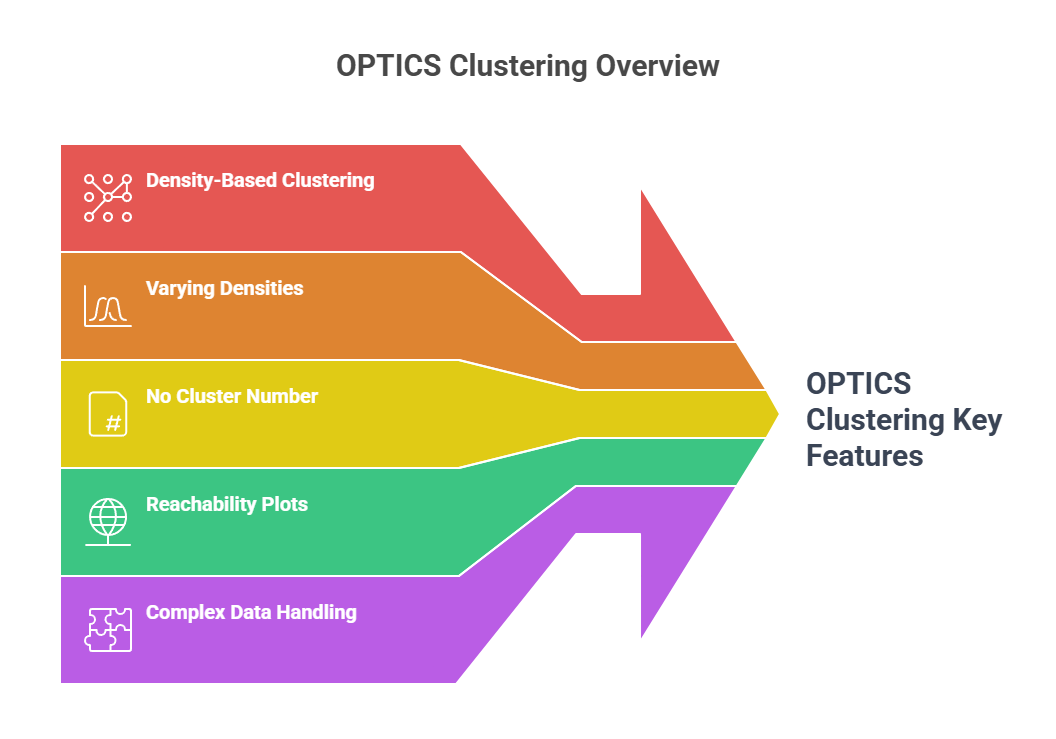
Key Features of OPTICS:
- No Need to Define the Number of Clusters: Unlike K-Means, which requires the number of clusters to be defined upfront, OPTICS automatically determines the number of clusters based on the data. This is beneficial when the true number of clusters in the data is unknown.
- Handling Varying Densities: One of the most important features of OPTICS is its ability to handle clusters with varying densities. It is designed to detect clusters of differing densities, making it well-suited for real-world datasets where clusters may not be uniformly distributed.
- Reachability Plots: OPTICS generates reachability plots, visually displaying the density-based relationships among data points. These plots provide insight into the structure of the clusters, making it easier to understand how data points are grouped based on their density.
Consider these carefully curated programs if you’re eager to deepen your knowledge and apply advanced AI and machine learning methods like OPTICS clustering. They are designed to equip you with practical skills and a strong grasp of the latest AI and ML developments:
- Master's in Artificial Intelligence and Machine Learning
- Executive Diploma in Machine Learning and AI
- Executive Post Graduate Certificate Programme in Data Science & AI
How OPTICS Differs from Other Clustering Algorithms
OPTICS clustering stands out due to its ability to handle clusters with varying densities and the fact that it doesn't require the user to specify the number of clusters in advance. This contrasts with algorithms like K-Means, which assume a predefined number of clusters and work best with clusters of similar density. DBSCAN, a density-based algorithm, can struggle with varying-density clusters. In contrast, OPTICS can uncover more nuanced clusters without being sensitive to noise and outliers.
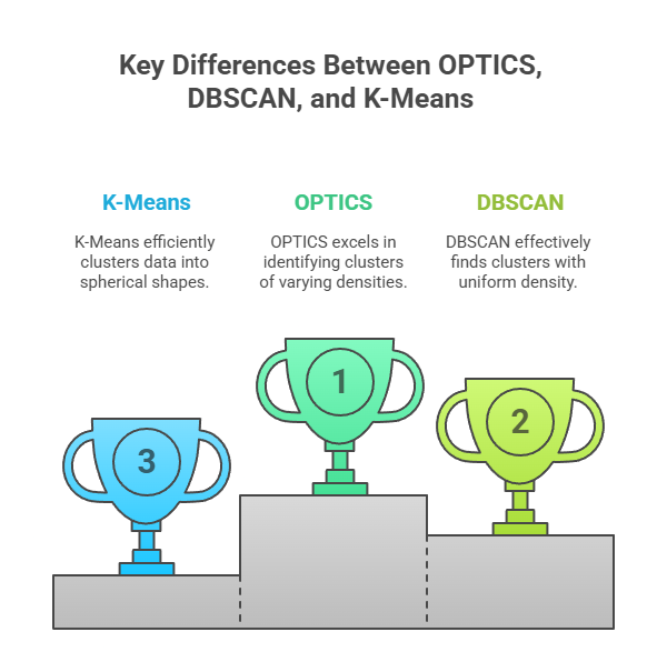
Key Differences Between OPTICS, DBSCAN, and K-Means
Understanding how OPTICS compares to DBSCAN and K-Means is crucial for selecting the algorithm for your clustering needs. Here's a breakdown of their key differences:
Feature | OPTICS | DBSCAN | K-Means |
Predefined Number of Clusters | No — automatically identifies clusters based on density ordering, without preset cluster count | No — identifies clusters based on density, no fixed number required | Yes — requires a predefined number of clusters (K) |
Handling Varying Densities | Handles clusters of varying densities by analyzing reachability distances | Best suited for clusters with similar densities; struggles with varying densities | Assumes clusters have similar densities and shapes |
Noise and Outlier Detection | Detects outliers based on reachability; not inherently superior to DBSCAN, but offers exploratory insight into cluster structure | Detects noise points effectively as outliers based on density threshold | Sensitive to noise; tends to assign outliers to nearest cluster, affecting accuracy |
Cluster Shape | Can identify clusters of arbitrary shape | Works well for non-convex, irregular shapes | Assumes spherical (convex) clusters |
Algorithm Type | Density-based, relies on reachability plot rather than fixed epsilon neighborhood | Density-based, requires fixed epsilon and minPts parameters | Centroid-based, optimizes distance to cluster centers |
Scalability | Computationally intensive due to reachability calculations; can be slower on very large datasets | May struggle with high-dimensional data; moderate scalability | Generally fast and scales well in time complexity, but performance degrades in high dimensions |
To better understand why OPTICS stands out among clustering methods, let’s explore how it compares to popular algorithms like K-Means and DBSCAN before diving into a step-by-step guide on how OPTICS works.
How Does the OPTICS Algorithm Work? A Step-by-Step Guide
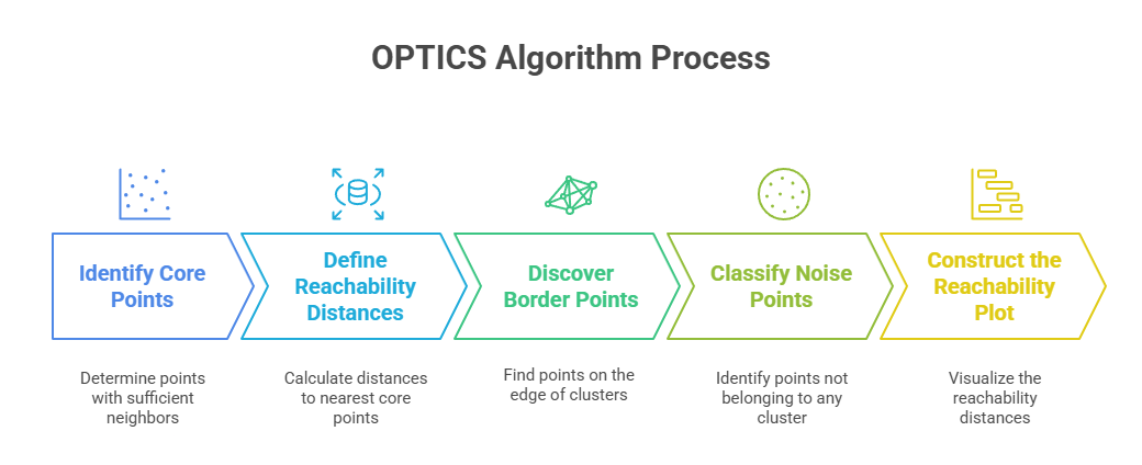
OPTICS (Ordering Points To Identify Clustering Structure) is a powerful algorithm in machine learning that overcomes several limitations of traditional clustering algorithms. It is designed to identify clusters of varying densities, eliminate the need to define the number of clusters, and detect noise efficiently. Below is a detailed breakdown of each key step in the OPTICS algorithm:
- Step 1: Identify Core Points
- A core point is a point that has a sufficient number of neighbors within a specified radius. This is determined by the parameters minPts (the minimum number of points within the radius) and epsilon (the radius size).
- Core points are central to the formation of clusters. They represent the center of a cluster. When a point is marked as core, all its neighbors within the epsilon radius are considered part of its cluster.
- Based on these parameters, the algorithm looks for all points directly reachable from a core point. A point cannot form a cluster if it does not meet this criterion.
- Step 2: Define Reachability Distances
- Reachability distance between two points pp and oo is defined as the maximum of the core distance of point oo and the direct distance between pp and oo.
- The core distance of oo represents how far oo is from its minPtsminPts nearest neighbors. The reachability distance essentially ensures that points are reachable if they are within the dense region defined by oo's neighborhood or closer.
- This measure helps build the reachability plot, which visually reveals the clustering structure in the data. Points with low reachability distances correspond to dense regions, while higher reachability distances indicate points near cluster edges or potential noise.
- Step 3: Discover Border Points
- Border points fall within the neighborhood of a core point but do not have enough neighbors to be considered core points themselves. These points are part of the cluster but not at its center.
- Border points are identified based on their proximity to core points. They help extend the cluster formed by the core points, providing a natural transition between different data groups.
- While border points contribute to the density of clusters, they are not the main representatives of the cluster's structure. They are necessary to ensure that the clusters are not artificially separated.
- Step 4: Classify Noise Points
- Noise points are the points that do not meet the criteria to be core or border points. Therefore, these points do not have enough neighbors within the epsilon radius to form a cluster and are considered outliers.
- Noise points can be seen in the reachability plot as isolated points with high reachability distances, indicating that they do not belong to any meaningful cluster.
- In practical terms, noise points represent data points that are either rare or irrelevant to the main structure of the data, and they are excluded from the final clusters.
- Step 5: Construct the Reachability Plot
- After processing all data points, OPTICS generates a reachability plot, a visual representation of the points and their corresponding reachability distances. This plot helps to identify the cluster structure, showing the density-based relationships between points.
- In the plot, clusters appear as regions with low and consistent reachability distances, while noise or outlier points are shown with large distances. The reachability plot allows for easy identification of clusters and their hierarchical structure.
- By analyzing the reachability plot, clusters can be defined by cutting the plot at a certain reachability threshold. This flexibility makes OPTICS particularly useful in exploratory data analysis, where the exact number of clusters is not known in advance.
Build your data analysis skills with the free Introduction to Data Analysis using Excel course. Learn how to clean, analyze, and visualize data using pivot tables, formulas, and more. Designed for beginners, this certification will enhance your analytical abilities and help you work more efficiently with data. Learn for free and start improving your data skills today!
Also read: Exploratory Data Analysis (EDA): Key Techniques and Its Role in Driving Business Insights
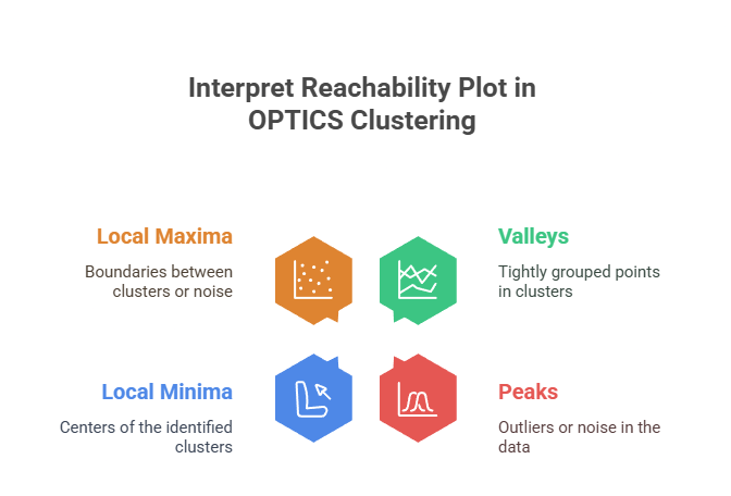
Reachability Plot in OPTICS Clustering
The reachability plot is one of the key features that sets OPTICS (Ordering Points To Identify Clustering Structure) apart from other clustering algorithms. It visually represents the density and structure of clusters, helping identify regions of high and low data density. Here's a deeper look into the role and interpretation of the reachability plot in OPTICS clustering:
- Role of Reachability Plot in OPTICS
The reachability plot displays the reachability distance for each data point, showing how far each point is from its nearest core point or cluster center. Low distances indicate dense regions, while high distances signal outliers. The plot highlights cluster structures and helps differentiate between dense clusters and sparse regions.
The plot aids in detecting dense regions and cluster boundaries by observing areas where reachability distances drop significantly. These drops mark local minima, which correspond to cluster centers. Conversely, local maxima indicate the transitions between clusters or points considered noise.
Also Read: Outlier Analysis in Data Mining: Techniques, Detection Methods, and Best Practices
- Interpreting the Reachability Plot
Clusters appear as valleys with low reachability distances, indicating tight groupings of data points. In contrast, outliers or noise points are represented by peaks with a high reachability distance. The boundary of each cluster is found by looking for sharp transitions in the plot.
- Example of Reachability Plot
For instance, when analyzing customer purchase data using OPTICS, the reachability plot can reveal dense customer segments (low valleys) and outlier behaviors (high peaks). By interpreting these features, you can identify key customer groups for targeted marketing strategies or detect unusual behaviors for fraud detection.
Core Points, Border Points, and Noise in OPTICS
The OPTICS algorithm categorizes points into core points, border points, and noise. These categories are essential for understanding how the algorithm identifies clusters and distinguishes outliers. Here’s a breakdown:
- Core Points
Core points are the backbone of a cluster. They have a sufficient number of neighboring points within a specified radius (determined by the MinPts parameter), indicating a dense region. These points help define where a cluster begins and ensure its continuity. Without core points, meaningful clusters cannot be formed.
- Border Points
Border points sit along the outer edge of a cluster. While they do not have enough neighbors to be core points themselves, they fall within the neighborhood of one or more core points. This connection assigns them to the cluster, even though they represent less dense areas. Border points help outline the shape and boundary of clusters.
- Noise Points
Noise points stand apart from clusters. They have too few neighbors to be core points and lie outside the neighborhood of any core point. These points are considered outliers or anomalies, often representing irregular or sparse data that does not fit into any cluster. Identifying noise is important for understanding data quality and removing irrelevant information.
If you’re ready to build a solid foundation in algorithms and data structures, join upGrad’s Data Structures & Algorithms course. In 50 hours, you’ll learn essential topics like algorithm analysis, searching and sorting, etc, all through expert-led online sessions. Plus, earn a recognized certification to demonstrate your skills and advance your career.
Also read: Comprehensive Guide on Density-Based Methods in ML
Implementing OPTICS Clustering with Python: A Walkthrough
This section will guide you through implementing OPTICS clustering using Python. We’ll use the popular Scikit-Learn library to perform clustering, followed by a detailed explanation of each code section. By the end, you’ll clearly understand how to apply OPTICS clustering to your datasets.
Example Code: Clustering Data Using OPTICS
from sklearn.cluster import OPTICS
import numpy as np
import matplotlib.pyplot as plt
# Create sample data
X = np.random.rand(100, 2)
# Apply OPTICS clustering
optics = OPTICS(min_samples=5, xi=0.05, min_cluster_size=0.1)
optics.fit(X)
# Plot the reachability plot
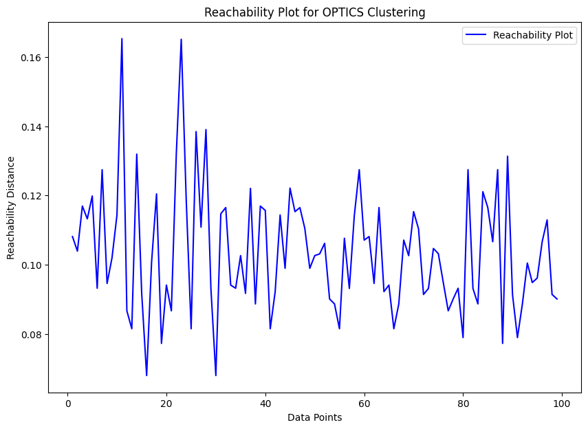
plt.figure(figsize=(10, 7))
plt.plot(range(len(X)), optics.reachability_, color='b', label='Reachability Plot')
plt.title('Reachability Plot for OPTICS Clustering')
plt.xlabel('Data Points')
plt.ylabel('Reachability Distance')
plt.legend()
plt.show()
# Visualizing the clusters
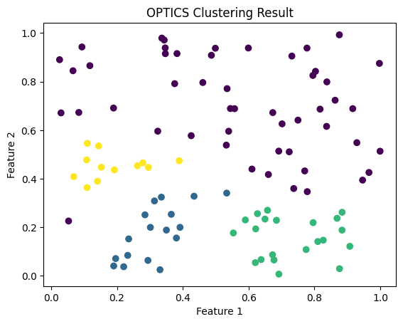
plt.scatter(X[:, 0], X[:, 1], c=optics.labels_, cmap='viridis')
plt.title('OPTICS Clustering Result')
plt.xlabel('Feature 1')
plt.ylabel('Feature 2')
plt.show()
Output:
-549879350327402aa46bd4a19aa9f9da.png)
Explanation of Code Sections:
- Import Libraries: We start by importing the necessary libraries—OPTICS from Scikit-Learn, numpy for data manipulation, and matplotlib for plotting.
- Data Generation: The np.random.rand() function generates random 2D data points to simulate clustering tasks.
- OPTICS Fit: The optics.fit() method applies the OPTICS algorithm to the generated data. We specify key parameters like min_samples, xi, and min_cluster_size to control clustering behavior.
- Reachability Plot: The reachability plot shows how the algorithm processes the data. It helps visualize the data point densities and their relationships during clustering.
- Cluster Visualization: Finally, we use plt.scatter() to plot the data points and color them based on the clusters identified by OPTICS.
Expected Output:
- The reachability plot will illustrate the clustering process, with data points on the x-axis and their respective reachability distances on the y-axis.
- The scatter plot will visualize the identified clusters, with different colors representing distinct groups of data points.
Visualizing OPTICS Clusters
Visualizing clusters formed by OPTICS is essential to understanding how the algorithm groups your data. In this section, we'll demonstrate how to visualize the clustering results, including the reachability plot and the final clusters.
How to Visualize Clusters:
- Reachability Plot: The reachability plot is an essential visualization for OPTICS clustering. It helps you understand the density and distribution of the data points, showing the order in which they were processed.
- Cluster Visualization: After clustering, it is crucial to visualize the data points grouped by their respective clusters. You can plot the clusters on a 2D space, colored by the cluster label, to visually inspect the results.
Example Python Code for Visualizing Clusters:
from sklearn.cluster import OPTICS
import numpy as np
import matplotlib.pyplot as plt
# Generate sample data
X = np.random.rand(100, 2)
# Apply OPTICS clustering
optics = OPTICS(min_samples=5, xi=0.05, min_cluster_size=0.1)
optics.fit(X)
# Visualize Reachability Plot
plt.figure(figsize=(10, 7))
plt.plot(range(len(X)), optics.reachability_, color='b', label='Reachability Plot')
plt.title('Reachability Plot for OPTICS Clustering')
plt.xlabel('Data Points')
plt.ylabel('Reachability Distance')
plt.legend()
plt.show()
# Visualizing Clusters
plt.figure(figsize=(10, 7))
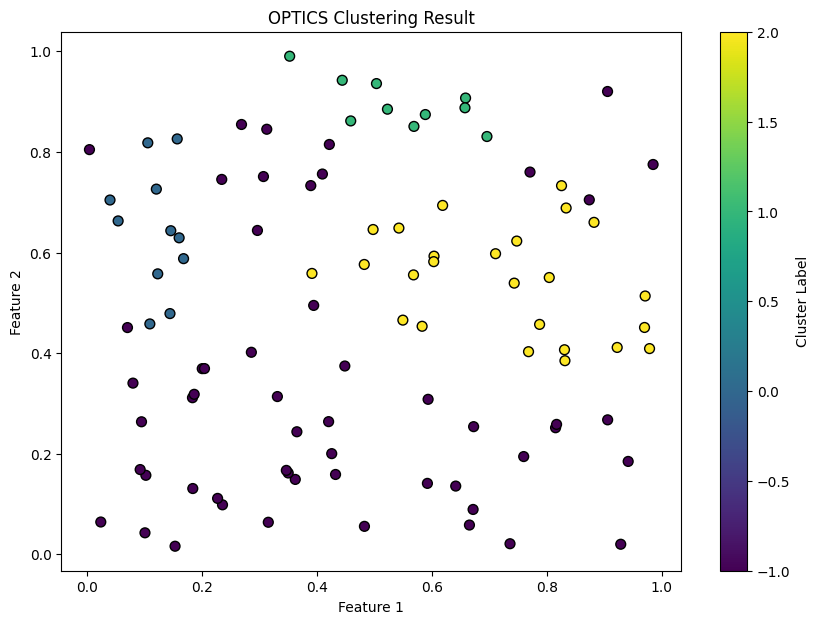
plt.scatter(X[:, 0], X[:, 1], c=optics.labels_, cmap='viridis', edgecolors='k', s=50)
plt.title('OPTICS Clustering Result')
plt.xlabel('Feature 1')
plt.ylabel('Feature 2')
plt.colorbar(label='Cluster Label')
plt.show()
Output:
Explanation of Code:
- The reachability plot visualizes the density-based ordering of data points, with valleys indicating dense clusters and peaks suggesting cluster boundaries or noise.
- The scatter plot shows data points colored by their assigned cluster labels, making it easy to see how OPTICS groups points of varying shapes and densities. Noise points are typically labeled as -1 and can be identified visually.
Also Read: Understanding the Role of Anomaly Detection in Data Mining
Applications of OPTICS Clustering in Machine Learning: Real-World Use Cases
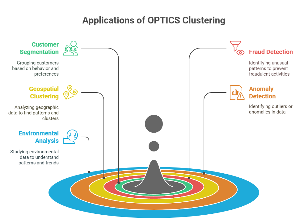
OPTICS clustering is widely used in various industries due to its ability to identify clusters of varying densities and handle noisy data. Below are some key applications where OPTICS proves to be highly effective:
- Customer Segmentation
In industries like retail and e-commerce, OPTICS clustering is used to segment customers based on purchasing behavior, demographics, or browsing patterns. Because customer segments often have irregular shapes and varying densities, OPTICS provides a more accurate way to identify these natural groupings.
Example: An e-commerce platform can segment customers into groups like frequent buyers, seasonal shoppers, and one-time purchasers, enabling tailored marketing and personalized recommendations.
- Anomaly Detection in Fraud Detection Systems
OPTICS is effective at detecting anomalous transactions or behaviors that deviate from normal patterns, which is crucial for fraud detection. Beyond simple outlier detection, OPTICS can identify rare clusters in complex, high-cardinality categorical data after embedding such features into continuous space, capturing subtle fraud patterns that traditional methods might miss.
Example: In banking, OPTICS can reveal fraudulent transactions by detecting unusual clusters or isolated points based on transaction amounts, locations, and times that differ from typical legitimate activity.
- Geospatial Data Clustering
OPTICS excels in clustering geospatial data where points are unevenly distributed and clusters vary in size and shape. This flexibility allows for better analysis of spatial relationships in applications like urban planning, retail site selection, and environmental studies.
Example: A real estate company can use OPTICS to identify areas with higher housing demand, while environmental agencies might cluster locations based on pollution levels or weather patterns to prioritize resource allocation and forecasting.
Ready to master unsupervised learning? upGrad's free Unsupervised Learning: Clustering course covers key techniques like K-Means and Hierarchical Clustering in just 11 hours. Learn practical Python applications and discover how to find hidden patterns in unlabelled data. Start building your skills today for free.
Also read: Difference Between Anomaly Detection and Outlier Detection
Now that we’ve covered the strengths and weaknesses of OPTICS clustering, let’s move on to a practical walkthrough of implementing this algorithm using Python and the Scikit-Learn library.
Advantages and Limitations of OPTICS Clustering: A Comprehensive Overview
This section provides an in-depth look at the advantages and limitations of OPTICS clustering, helping you understand when and why to use it and its potential challenges.
Advantages of OPTICS Clustering
OPTICS clustering offers several benefits that make it suitable for real-world applications where traditional clustering methods fall short.
- Effectively identifies clusters with varying densities and arbitrary shapes, providing flexibility beyond algorithms like K-Means.
- Detects noise and outliers by distinguishing sparse regions from dense clusters, improving pattern relevance.
- Produces a reachability plot that visually reveals the cluster hierarchy and structure, aiding interpretability and decision-making.
Limitations of OPTICS Clustering
While OPTICS has several advantages, it has certain limitations that should be considered when choosing it for specific applications.
- Computationally intensive on large datasets due to repeated distance calculations, which can limit scalability and real-time applicability.
- Sensitive to the choice of distance metrics and parameters; selecting appropriate measures is crucial for meaningful clusters.
- Performance may decline with very high-dimensional data unless combined with dimensionality reduction techniques like PCA or t-SNE to improve efficiency and accuracy.
Here’s a comparison of the key advantages and limitations of OPTICS clustering to help you assess its suitability for your data analysis needs:
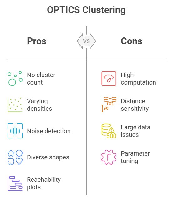
Advantages | Limitations |
Handles varying densities and cluster shapes | High computational cost on large datasets |
Detects noise and outliers effectively | Sensitive to distance metrics and parameter settings |
Provides reachability plots for insight | May require dimensionality reduction for high-dimensional data |
Want to turn data into compelling stories? upGrad’s free Analyzing Patterns in Data and Storytelling course teaches you how to identify patterns, create insights, and use data visualization effectively. In just 6 hours, learn key techniques like the Pyramid Principle and logical flow to make your data clear and impactful.
Also read: Machine Learning Tutorial: Learn ML from Scratch
Test Your Knowledge of OPTICS Clustering with a Quiz
Test your understanding of OPTICS Clustering with the following quiz. This set of multiple-choice questions will help you gauge your knowledge about the algorithm, its functionality, and its applications in various fields.
- What is the main advantage of OPTICS over K-Means?
- a) No need to predefine the number of clusters
- b) Faster convergence
- c) Works only with spherical clusters
- d) Can only handle numeric data
- Which of the following is a key feature of the OPTICS algorithm?
- a) Fixed number of clusters
- b) Use of reachability plots
- c) Works only with linear data
- d) Requires manual cluster labeling
- In OPTICS, what does the reachability distance represent?
- a) The distance between two data points
- b) The time taken for the algorithm to reach a cluster
- c) The density relationship between data points
- d) The distance between a point and the nearest cluster center
- What type of data is OPTICS clustering best suited for?
- a) Linear data
- b) Data with arbitrary shapes and varying densities
- c) Text data
- d) Data with a fixed number of clusters
- Which of the following clustering algorithms is often compared to OPTICS?
- a) K-Means
- b) Linear Regression
- c) Random Forest
- d) Logistic Regression
- How does OPTICS handle noise in data?
- It assigns noise points to the nearest cluster
- It ignores noise points when forming clusters but retains them in the dataset
- It treats noise as part of a cluster
- It removes noise points from the dataset entirely
- Which of the following is NOT a common application of OPTICS clustering?
- a) Customer segmentation
- b) Image compression
- c) Anomaly detection
- d) Geospatial data clustering
- What does the 'min_samples' parameter in OPTICS control?
- a) The maximum number of clusters
- b) The minimum number of points required to form a cluster
- c) The density threshold for outlier detection
- d) The distance between clusters
- Which of the following is an advantage of OPTICS over DBSCAN?
- a) Requires less computational power
- b) Does not require the density threshold
- c) Can find clusters of varying shapes and densities
- d) More intuitive for small datasets
- Which Python library is commonly used to implement OPTICS clustering?
- a) Pandas
- b) Scikit-learn
- c) TensorFlow
- d) PyTorch
Now that you’ve tested your OPTICS knowledge, explore more clustering techniques and enhance your skills with upGrad’s expert-led courses.
Learn More Clustering Techniques with upGrad
OPTICS clustering groups data by identifying clusters of varying densities without needing a preset number of clusters. Its reachability plots and flexible noise handling suit complex datasets where traditional methods struggle.
Though more computationally intensive, OPTICS’ ability to uncover natural clusters in diverse data makes it valuable for data professionals. Mastery requires hands-on experience beyond theory.
upGrad’s carefully designed programs guide you through real-world applications of clustering methods, including OPTICS. You’ll learn how to apply these techniques effectively to solve challenging data problems through hands-on projects, case studies, and expert mentorship.
Explore these courses to deepen your understanding and boost your career:
Besides the courses above, upGrad also offers free courses that you can use to get started with the basics:
- Artificial Intelligence in the Real World
- Data Science in E-commerce
- Linear Regression - Step by Step Guide
- Introduction to Natural Language Processing Free Courses
Not sure how to move forward in your ML career? upGrad provides personalized career counseling to help you choose the best path based on your goals and experience. Visit a nearby upGrad centre or start online with expert-led guidance.
FAQs
1. How does OPTICS reveal cluster hierarchy without explicit cluster assignments?
OPTICS orders data points based on reachability distances instead of fixed labels, capturing the density-based structure and hierarchy. This ordering allows flexible cluster extraction at different density levels by analyzing the reachability plot, supporting multi-scale exploration without preset cluster numbers. This makes OPTICS especially useful for exploratory data analysis where cluster boundaries aren’t well defined.
2. What role do the ‘xi’ and ‘min_samples’ parameters play in OPTICS?
The ‘xi’ parameter controls the sensitivity to changes in reachability distances, helping identify cluster boundaries by balancing detection of small detailed clusters versus broader groups. ‘min_samples’ sets the minimum neighbors for a core point, affecting cluster density requirements. Tuning these often involves combining domain knowledge with visual inspection of the reachability plot and metrics like silhouette scores to optimize clustering quality. Proper parameter tuning is crucial to avoid over- or under-clustering.
3. How does OPTICS handle noise and outliers in data?
Noise points are identified as those with high reachability distances that fall outside dense regions. OPTICS excludes these from clusters but retains them in the dataset for separate analysis, improving cluster clarity and model accuracy by focusing on meaningful structures. This selective noise handling helps maintain robust clustering results even in noisy datasets.
4. Can OPTICS manage clusters with varying densities, shapes, and sizes?
Yes, OPTICS’s density-based approach and use of reachability distances enable it to detect clusters regardless of shape or size, including elongated or nested clusters. This flexibility surpasses centroid-based methods, making OPTICS suitable for complex real-world data distributions. As a result, it adapts well to datasets where cluster structures are irregular and non-convex.
5. How does OPTICS perform on high-dimensional or large datasets, and how can challenges be mitigated?
OPTICS can struggle with high-dimensional data due to distance metric degradation and increased computational cost. Dimensionality reduction methods (e.g., PCA, t-SNE) often improve results. For large datasets, the main bottleneck is computing neighborhoods and updating reachability distances, which scales poorly. Using spatial indexing structures like ball trees or approximate nearest neighbor algorithms can significantly reduce runtime. Combining these approaches helps make OPTICS practical for bigger and more complex datasets. OPTICS can struggle with high-dimensional data due to distance metric degradation and increased computational cost. Dimensionality reduction methods (e.g., PCA , t-SNE) often improve results. For large datasets, the main bottleneck is computing neighborhoods and updating reachability distances, which scales poorly. Using spatial indexing structures like ball trees or approximate nearest neighbor algorithms can significantly reduce runtime. Combining these approaches helps make OPTICS practical for bigger and more complex datasets.
6. How can OPTICS clustering be integrated with other machine learning techniques?
The reachability plot and cluster labels from OPTICS serve as valuable features for supervised learning, anomaly detection, and data segmentation. OPTICS pairs well with dimensionality reduction and visualization techniques, and in fields like time series or spatial analysis, it helps isolate meaningful segments before applying predictive models. This integration enhances the overall performance and interpretability of machine learning workflows. The reachability plot and cluster labels from OPTICS serve as valuable features for supervised learning , anomaly detection, and data segmentation. OPTICS pairs well with dimensionality reduction and visualization techniques, and in fields like time series or spatial analysis, it helps isolate meaningful segments before applying predictive models. This integration enhances the overall performance and interpretability of machine learning workflows.
7. What are practical strategies for tuning OPTICS parameters effectively?
Begin with domain knowledge to set initial ‘min_samples’ and ‘xi’ values. Use the reachability plot for visual feedback, looking for clear valleys indicating clusters. Quantitative metrics such as silhouette scores or elbow methods can aid in balancing cluster granularity, noise filtering, and computational efficiency. Iterative experimentation with distance metrics also helps refine results. Careful tuning ensures OPTICS reveals meaningful patterns without excessive fragmentation or merging.
8. What is the significance of the reachability distance in OPTICS?
Reachability distance measures how close a point is to its neighbors considering local density, combining core distance and actual distance. It forms the foundation of the reachability plot, enabling identification of cluster structures and density variations. Understanding reachability distance is key to interpreting how OPTICS separates dense clusters from noise. This measure also allows OPTICS to adaptively capture clusters at multiple density levels without fixed parameters.
9. How does OPTICS differ from DBSCAN in handling clusters of different densities?
Unlike DBSCAN, which uses a fixed density threshold, OPTICS creates an ordering of points that reflects clustering at multiple density levels. This makes OPTICS better suited for datasets with clusters of varying densities, where DBSCAN may merge or miss clusters. The flexibility of OPTICS allows users to extract clusters at different granularities post-processing. Consequently, OPTICS provides more detailed insights into the data's intrinsic clustering structure.
10. Can OPTICS handle categorical or mixed-type data?
OPTICS is primarily designed for numerical data using distance metrics like Euclidean distance. For categorical or mixed data types, preprocessing steps such as embedding or converting categories into numerical vectors are required. After transformation, OPTICS can cluster such data effectively, although careful metric selection remains critical. However, the quality of embeddings significantly impacts clustering performance and interpretability.
11. I’m overwhelmed by all the clustering options and unsure if OPTICS is right for my data. How can I get help to choose and apply the best method?
Choosing the right clustering algorithm can be confusing, especially with complex data and multiple parameters to tune. Getting expert counseling or visiting an offline center can provide personalized guidance tailored to your dataset and goals. This support ensures you select the most effective method, understand its implementation, and avoid costly trial-and-error.


upGrad Learner Support
Talk to our experts. We are available 7 days a week, 10 AM to 7 PM
Indian Nationals
Foreign Nationals
