All courses
Agentic AI
Agentic AI

IIIT Bangalore
Executive Programme in Generative AI for LeadersArtificial Intelligence
Degree / Exec. PG

IIIT Bangalore
Executive Diploma in Machine Learning and AI
OPJ Global University
Master’s Degree in Artificial Intelligence and Data Science
Liverpool John Moores University
Master of Science in Machine Learning & AI
Golden Gate University
DBA in Emerging Technologies with Concentration in Generative AIExecutive Certificate

IIITB & IIM, Udaipur
Chief Technology Officer & AI Leadership ProgrammeIIIT Bangalore
Executive Programme in Generative AI for Leaders
upGrad | Microsoft
Gen AI Foundations Certificate Program from MicrosoftupGrad | Microsoft
Gen AI Mastery Certificate for Data AnalysisupGrad | Microsoft
Gen AI Mastery Certificate for Software DevelopmentupGrad | Microsoft
Gen AI Mastery Certificate for Managerial ExcellenceOffline Bootcamps

upGrad
Data Science and AI-MLDoctorate
For All Domains
IIITB & IIM, Udaipur
Chief Technology Officer & AI Leadership Programme
Swiss School of Business and Management
Global Doctor of Business Administration from SSBM
Edgewood University
Doctorate in Business Administration by Edgewood UniversityGolden Gate University
Doctor of Business Administration From Golden Gate University
Rushford Business School
Doctor of Business Administration from Rushford Business School, SwitzerlandGolden Gate University
Master + Doctor of Business Administration (MBA+DBA)-d9bdeff6165f4eb1ba2adcebde78e961.svg)
University of Waterloo
Chief Technology and AI Officer ProgramLeadership / AI
Golden Gate University
DBA in Emerging Technologies with Concentration in Generative AIMachine Learning
Machine Learning
Data Science
Degree / Exec. PG
O.P Jindal Global University
Master’s Degree in Artificial Intelligence and Data ScienceIIIT Bangalore
Executive Diploma in Data Science & AILiverpool John Moores University
Master of Science in Data ScienceExecutive Certificate
upGrad | Microsoft
Gen AI Foundations Certificate Program from MicrosoftupGrad | Microsoft
Gen AI Mastery Certificate for Data AnalysisupGrad | Microsoft
Gen AI Mastery Certificate for Software DevelopmentupGrad | Microsoft
Gen AI Mastery Certificate for Managerial ExcellenceupGrad | Microsoft
Gen AI Mastery Certificate for Content CreationOffline Bootcamps
upGrad
Data Science and AI-MLupGrad
Data AnalyticsMBA
Masters

Paris School of Business
Master of Science in Business Management and TechnologyO.P.Jindal Global University
MBA (with Career Acceleration Program by upGrad)Edgewood University
MBA from Edgewood UniversityO.P.Jindal Global University
MBA from O.P.Jindal Global UniversityGolden Gate University
Master + Doctor of Business Administration (MBA+DBA)Executive Certificate

IMT, Ghaziabad
Advanced General Management ProgramMarketing
Executive Certificate
Offline Bootcamps
upGrad
Digital MarketingManagement
Degree
O.P Jindal Global University
MSc in International Accounting & Finance (ACCA integrated)Paris School of Business
Master of Science in Business Management and Technology
Golden Gate University
Master of Arts in Industrial-Organizational PsychologyExecutive Certificate

IIIT-B & IIM, Udaipur
Chief Technology Officer & AI Leadership Programme
IIM Kozhikode
Human Resource Analytics Course from IIM-KupGrad | Microsoft
Gen AI Foundations Certificate Program from MicrosoftEducation
Education

Northeastern University
Master of Education (M.Ed.) from Northeastern UniversityEdgewood University
Doctor of Education (Ed.D.)Edgewood University
Master of Education (M.Ed.) from Edgewood UniversityCertifications
Project Management
Certification

Knowledgehut
Leadership And Communications In ProjectsKnowledgehut
Microsoft Project 2007/2010-ae8d039bbd2a41318308f8d26b52ac8f.svg)
Knowledgehut
Financial Management For Project ManagersKnowledgehut
Fundamentals of Earned Value Management (EVM)Knowledgehut
Fundamentals of Portfolio ManagementKnowledgehut
Fundamentals of Program Management-35c169da468a4cc481c6a8505a74826d.webp&w=128&q=75)
Knowledgehut
CAPM® CertificationsKnowledgehut
Microsoft® Project 2016Certifications & Trainings
-7f4b4f34e09d42bfa73b58f4a230cffa.webp&w=128&q=75)
Knowledgehut
PMP® CertificationKnowledgehut
PMI-RMP® CertificationKnowledgehut
PMP Renewal Learning PathKnowledgehut
Oracle Primavera P6 V18.8Knowledgehut
Microsoft® Project 2013Knowledgehut
PfMP® Certification CourseKnowledgehut
Project Planning and MonitoringPrince2 Certifications

Knowledgehut
PRINCE2® FoundationKnowledgehut
PRINCE2® PractitionerKnowledgehut
PRINCE2 Agile Foundation and PractitionerKnowledgehut
PRINCE2 Agile® Foundation CertificationKnowledgehut
PRINCE2 Agile® Practitioner CertificationManagement Certifications
Knowledgehut
Project Management Masters Certification ProgramKnowledgehut
Change ManagementKnowledgehut
Project Management TechniquesKnowledgehut
Product Management Certification ProgramKnowledgehut
Project Risk Management- Study abroad
- Offline centres
- uGSOT - B.Tech
More


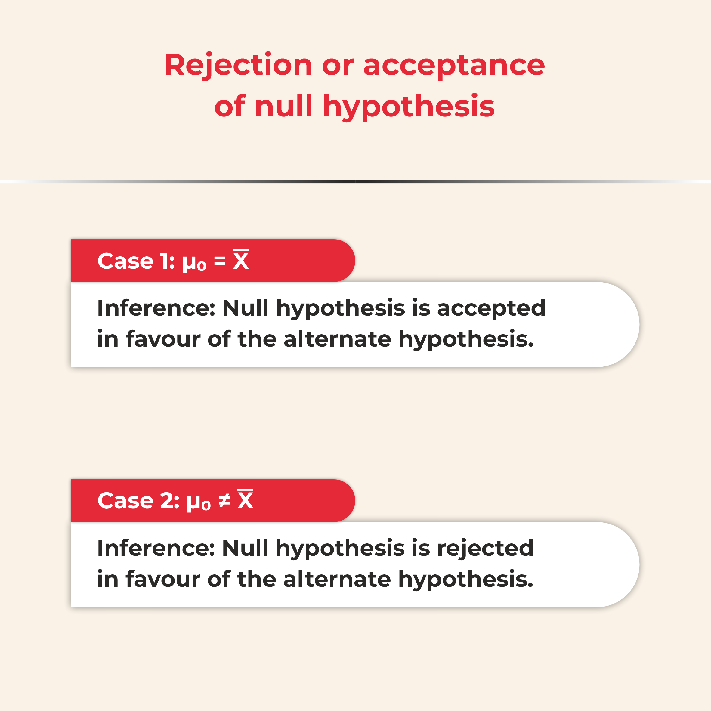
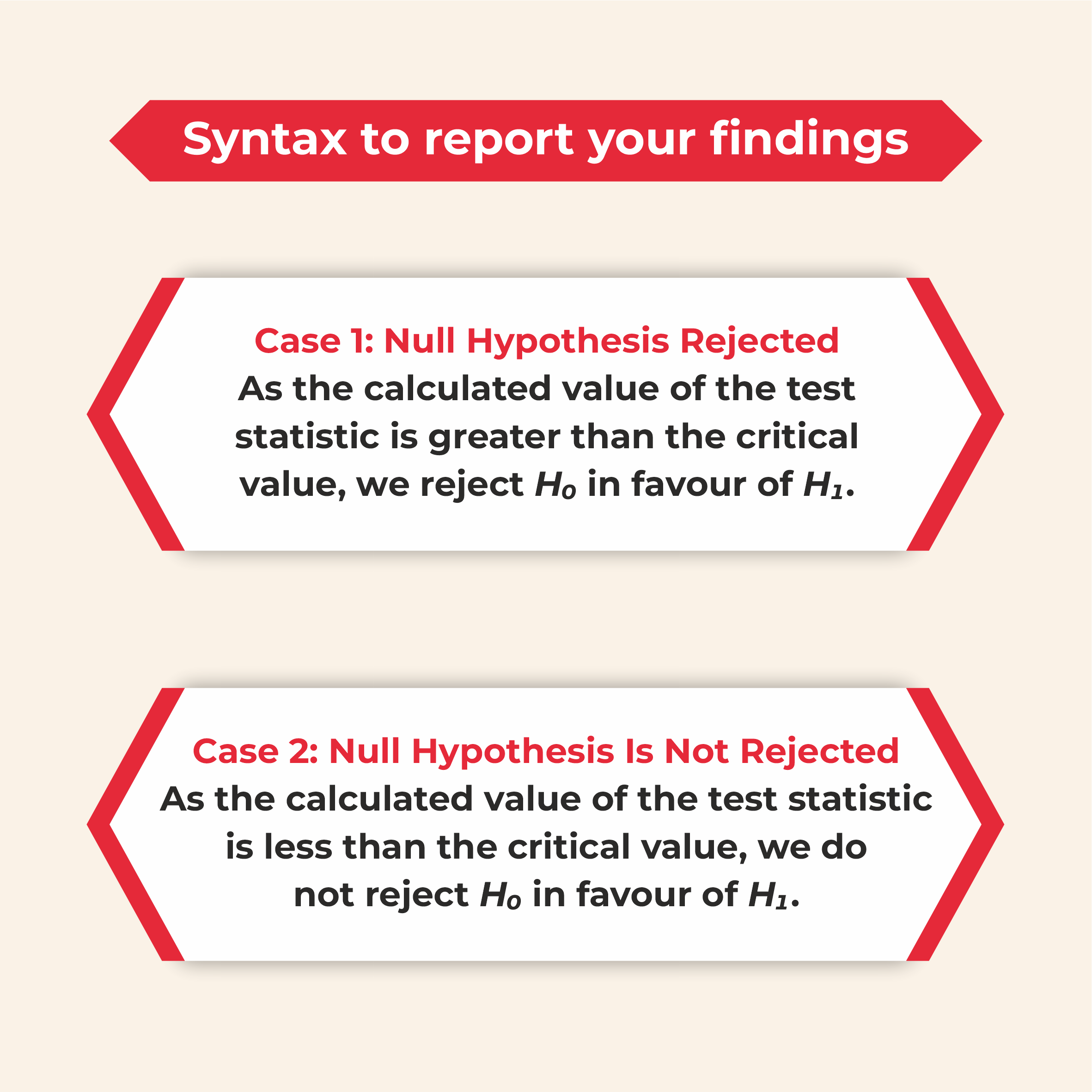
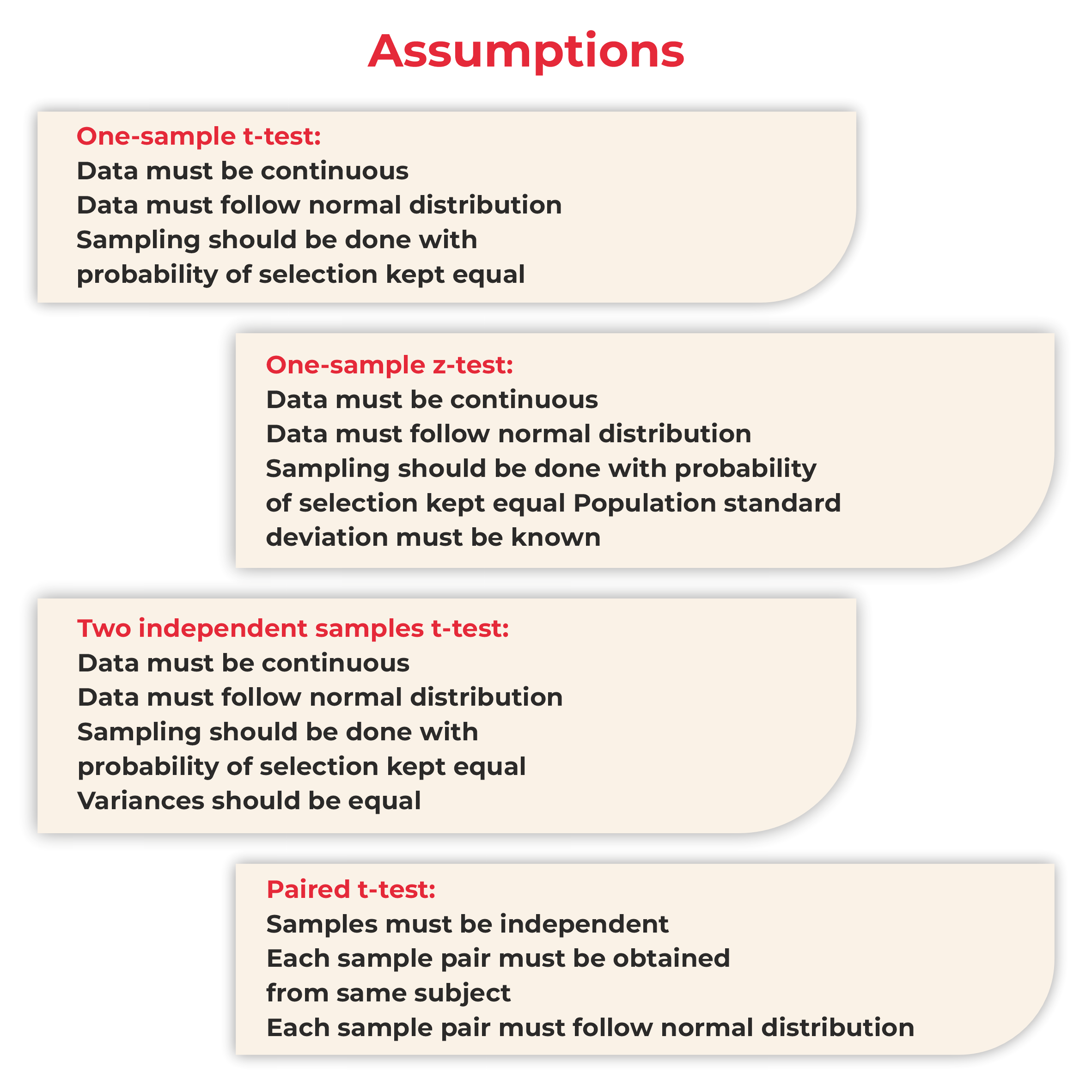
Hypothesis Testing Courses Online
Hypothesis Testing Courses provide practical training in statistical inference, helping you understand p-values, t-tests, ANOVA, and confidence intervals. You’ll learn how to analyze data, validate assumptions, and make confident, data-driven decisions for business, research, and analytics roles.
-80f5aca04e9b49ca9902fe2806c12f6e%20(1)-05c9b5b2614c40b681f04c3275487b40.jpeg&w=3840&q=75)
Hypothesis Testing Course Overview
Hypothesis testing is one of the most pivotal concepts in statistics with many real-life applications. It is used by researchers all over the world to test new theories before implementing them. It helps different companies set a baseline quality of their product and decide on improvements.
There are a lot of different parts of testing a hypothesis, from creating a statistical statement to calculations. Nowadays, most of the work in this field is done using software like python, Minitab, SQL, or R.
Apart from using software, testing problems can also be solved by hand, though the process would be time-consuming and tedious.
Hypothesis Testing Course Instructors
Learn From The Best
Learn Hypothesis Testing from expert instructors who help you excel in your careers by imparting cutting-edge analytics and machine learning skills.
8
Instructors
10
Industry Experts


-39a9e7a7278a441ea08a60a1f45b4913.png&w=128&q=75)


Placements in Hypothesis Testing Courses
Our Placement Numbers
Excel in data-driven careers with our Hypothesis Testing Courses, boasting a high rate of successful student placements. Get hired by top companies.
Top Recruiters


Success Stories
What Our Learners Have To Say


Learner Support and Services
How Will upGrad Supports You
Receive unparalleled guidance from industry mentors, teaching assistants, and graders
Receive one-on-one feedback from our seasoned data science faculty on submissions and personalized feedback to improvement
Our Data Science Syllabus is designed to provide you with ample of industry relevant knowledge with examples
FAQs about Hypothesis Testing Course
1. What is the use of hypothesis testing in real life?
Real-life hypothesis testing allows researchers to test new theories before implementing them. It is used in different industries to set standards for their products. It is especially helpful to statisticians when designing an experiment with many parameters.
2. What is the difference between simple and composite hypotheses?
Statistical hypotheses are of two types. Simple and composite.
A statistical hypothesis that specifies the distribution of the parent population from which the random samples to be used for testing has been generated is known as a simple hypothesis.
A statistical hypothesis that does not specify the distribution of the parent population from which the random samples to be used for testing has been generated is known as a composite hypothesis.
3. What statistical concepts are needed to get a good grasp on hypothesis testing?
One needs to know probability theory, the different types of probability distributions, and statical inference to get a good grasp on the testing of a hypothesis.


upGrad Learner Support
Talk to our experts. We are available 7 days a week, 10 AM to 7 PM
Indian Nationals
Foreign Nationals
Disclaimer
The above statistics depend on various factors and individual results may vary. Past performance is no guarantee of future results.
The student assumes full responsibility for all expenses associated with visas, travel, & related costs. upGrad does not .