Mean Shift Clustering: How the Algorithm Groups Data Without Predefined K

Mean shift clustering is a machine learning technique that groups data points without needing a predefined number of clusters (K).  Unlike algorithms like K-Means, which require K to be set in advance, Mean Shift dynamically determines the optimal number of clusters based on the data's distribution. This makes it ideal for complex, non-linear data patterns. 

In this blog, we will explore how Mean Shift works, its key features, and its practical applications in real-world machine learning tasks.

Advance your AI and ML skills with expert courses by upGrad, designed by top global universities. Explore Data Science, Deep Learning, NLP, and more. Learn core concepts like epochs in machine learning and apply them in real-world settings.

What Is Mean Shift Clustering and Why It Matters? Core Concepts

Mean shift clustering is a powerful, non-parametric clustering technique that helps group data points based on the highest density regions in the data. Unlike traditional clustering methods like K-Means, the Mean Shift Algorithm does not require predefined cluster numbers (K), making it ideal for complex, non-linear data distributions. 

Key Concepts:

• Mode: In mean shift clustering, the mode refers to the point of highest data density, representing a "peak" in the dataset. It is where data points are most concentrated. Identifying modes helps group data effectively by focusing on regions with higher likelihoods of belonging to the same cluster.
• Density Estimation: Density is estimated using a kernel function that assigns a weight to each data point based on its distance from others. This helps identify the densest regions in the data. The kernel function, often a Gaussian, smooths the data, allowing the algorithm to locate the peaks or modes where clusters naturally form.
• Iterative Shifting: The mean shift algorithm works by iteratively shifting data points toward the mode. With each iteration, data points move towards the highest density until convergence is achieved, meaning the points stop shifting once they settle at a mode. This process refines the position of each cluster, ensuring that data points are grouped correctly.

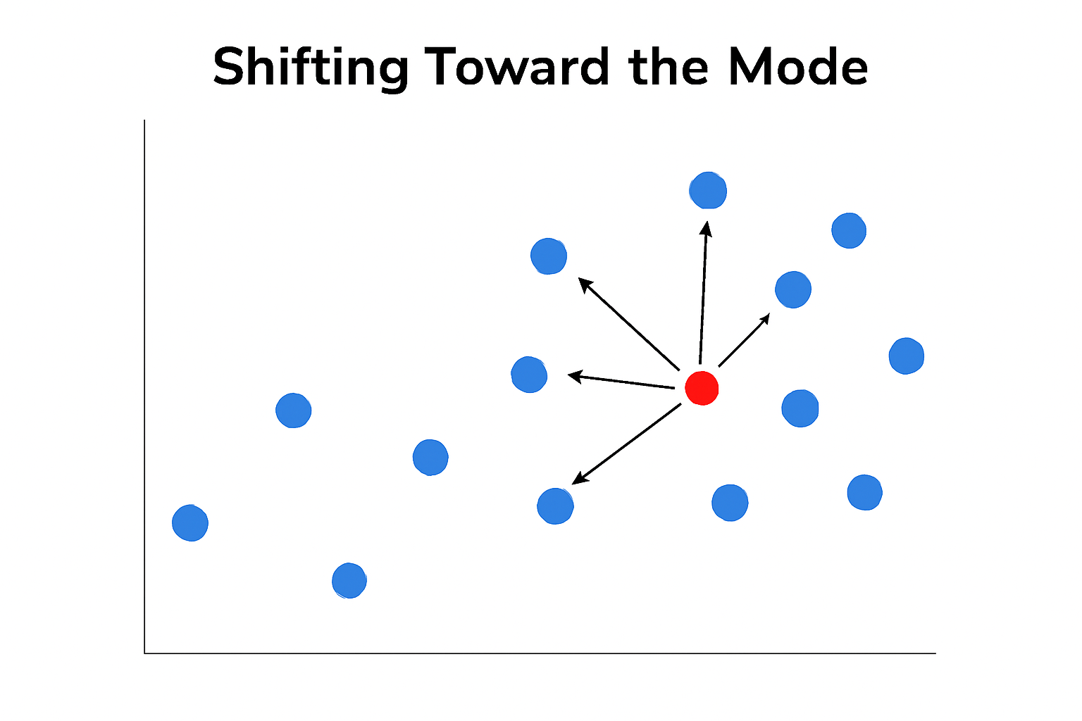
• Comparison to Gravity: The iterative shifting process in mean shift clustering can be compared to gravity or hill climbing. Like how an object moves toward a gravitational pull or climbs to the top of a hill, data points in the mean shift algorithm shift towards the mode, identifying the densest region in the data and ultimately converging at the peak.
• No Fixed cluster centers: Unlike algorithms such as K-Means, which rely on fixed cluster centers, the mean shift algorithm adapts dynamically to the data. The "centroids" are not predefined but evolve throughout the clustering process, allowing for more accurate and flexible clustering without requiring a specified number of clusters.

Why It Matters:

Mean shift clustering provides a more adaptable and precise approach to clustering complex data. Not requiring predefined clusters and dynamically adapting to data distributions helps uncover meaningful patterns that other methods, such as K-Means, may miss. 

This flexibility is essential in exploratory data analysis, where the true number of clusters is unknown, allowing analysts to discover clusters based on actual data patterns rather than predefined assumptions.

Ready to deepen your knowledge of AI and ML? Here are some highly-rated courses to elevate your expertise and take on advanced techniques:

• Executive Diploma in Machine Learning and AI
• Master's in Artificial Intelligence and Machine Learning
• Executive Post Graduate Certificate Programme in Data Science & AI

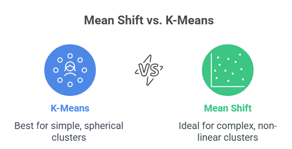
Mean Shift vs. Other Clustering Methods like K-Means

Mean shift clustering offers a flexible approach compared to methods like K-Means. Unlike K-Means, which assumes spherical clusters and requires predefined K, mean shift automatically adapts to data distributions, detecting clusters based on density peaks. This flexibility is ideal for complex, non-linear data, eliminating the need to guess the number of clusters.

• K-Means Assumptions: K-Means assumes clusters are spherical and requires a predefined number of clusters (K). It works by partitioning data into K clusters based on proximity to cluster centers. However, it struggles with irregular-shaped or unequal-sized clusters and can give misleading results if K is incorrectly set.
• Mean Shift's Flexibility: Unlike K-Means, mean shift does not assume a specific shape or number of clusters. It finds clusters based on density peaks, making it ideal for varied data distributions. This flexibility allows it to detect arbitrarily shaped clusters, leading to more accurate results in complex datasets.
• Adapting to Data Distribution: While K-Means forces data into predefined shapes, mean shift automatically adjusts to the data's underlying structure. Shifting points toward regions of high data density groups data in a way that better reflects real-world distributions.
• When to Use Which Method: K-Means is efficient when you know the number of clusters and expect spherical groupings. Mean shift offers greater adaptability for complex, non-linear datasets with unknown cluster shapes.

Also Read: Difference Between Linear and Non-Linear Data Structures

Overcoming K-Means Limitations with Mean Shift Clustering

One of the most significant challenges in clustering with K-Means is selecting the optimal K. The choice of K can majorly impact the model's effectiveness, and improper selection can lead to poor results.

Unlike K-Means, mean shift clustering automatically detects clusters by identifying density peaks in the data. This eliminates the need to specify the number of clusters beforehand, making it more adaptable to exploratory data analysis, where the true cluster structure is unknown.

• Benefits for Exploratory Data Analysis: Mean shift benefits exploratory data analysis. This allows analysts to uncover hidden patterns and gain insights without the risk of arbitrarily choosing an incorrect K value.
• Example: Imagine analyzing customer purchase data in an e-commerce platform. K-Means might require you to set the number of customer segments in advance. In contrast, Mean shift automatically groups customers based on their purchasing behavior, revealing patterns that would otherwise be missed, such as a niche segment of highly loyal customers.

Comparison Table: Mean Shift vs K-Means

This table highlights the key differences between mean shift and K-Means clustering algorithms, focusing on flexibility, handling of clusters, and when each method is most effective.

By highlighting the differences between mean shift and traditional clustering methods like K-Means, it’s clear that mean shift clustering is a more adaptable method for non-linear and complex data sets. This makes it particularly useful in fields like image segmentation, where clusters may have irregular shapes, and in geographic data analysis, where data distributions are often uneven and unpredictable.

If you're looking to master more than flexible clustering techniques, upGrad's Fundamentals of Deep Learning and Neural Networks course is the perfect fit. In just 28 hours, you'll explore key concepts, helping you adapt AI models to complex data. Plus, earn a signed, verifiable e-certificate from upGrad.

Also read: 17 AI Challenges in 2025: How to Overcome Artificial Intelligence Concerns?

Now that you’ve explored the core concepts of mean shift clustering and compared it with other methods like K-Means, let’s dive into how the algorithm works step by step.

How the Mean Shift Algorithm Works Step by Step

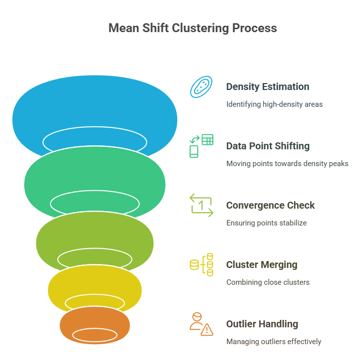
The mean shift algorithm iteratively shifts data points toward high-density areas, forming clusters without predefined K values. It uses a kernel and bandwidth to smooth data and detect modes (peaks in data density) until convergence, making it ideal for complex data distributions.

1. Defining the Kernel and Bandwidth 

In the mean shift algorithm, the kernel function defines how data points are weighted within their local neighborhood, determining the shape and influence of each neighborhood. Commonly used kernels include the Gaussian kernel, which assigns higher weights to points closer to the center and lower weights to points farther away.

• Kernel Function: Specifies how points within a neighborhood influence each other, ensuring the shift occurs towards the density peak. The choice of kernel affects how well the algorithm adapts to different data structures. For example, a Gaussian kernel is suitable for smooth data distributions, while other kernels, such as the Epanechnikov kernel, are better for compact clusters.
• Bandwidth: A crucial parameter that determines the radius of the neighborhood. A larger bandwidth smooths the data more widely, while a smaller bandwidth focuses on finer, local structures. The selection of the right bandwidth is critical as it influences the sensitivity of the clustering. A large bandwidth may over-smooth data and merge distinct clusters, while a small bandwidth can create too many small clusters or noise.
• Effect: Together, the kernel and bandwidth define how the data's density is estimated. The kernel determines the weight each point receives in the shifting process, and the bandwidth controls the neighborhood size, both impacting the clustering's accuracy and speed.

Also read: Gaussian Naive Bayes: Understanding the Algorithm and Its Classifier Applications

2. Iterative Shifting of Data Points Toward Cluster Centers

Mean shift works by shifting each data point toward the average (mean) of its local neighborhood, iterating until the data points converge around high-density areas. This process ensures that the points group around regions of maximum data density, referred to as modes (local density peaks).

• Shifting Process: In each iteration, points are shifted towards higher-density regions, gradually converging towards the densest modes. This ensures that points end up in clusters corresponding to the densest areas of data.
• Iteration: The shifting is repeated until the movement between successive iterations becomes negligible, signaling convergence and stable clusters. This iterative process is robust and effective, even for complex, multi-modal data distributions.
• Density Role: The algorithm places greater emphasis on regions with higher data density, ensuring that data points are pulled more strongly toward the centers of modes. This makes mean shift highly adaptable to varying data distributions.

Example: Consider a set of data points in a 2D space. Each point shifts towards the peak of the highest-density region until the entire group converges, forming a cluster around that mode.

3. Convergence Criteria and Final Cluster Formation 

The algorithm stops when shifts become minimal, indicating that data points have converged to their corresponding modes, effectively forming clusters.

• Stopping Criterion: The algorithm halts when the shift of data points between iterations is minimal, signaling that the points have converged and stable clusters have formed.
• Cluster Formation: Data points that converge near the same mode are grouped together into one cluster. These clusters represent the densest regions in the data, with each mode representing a separate group of similar points.
• Pruning/Merging: If clusters are too close to each other, they may be merged to form a more accurate grouping. This step ensures that clusters are well-defined and reduces the risk of over-segmentation.
• Noise Handling: Points that converge to modes with insufficient data density—often outliers—are either ignored or pruned. This ensures that the final clusters reflect meaningful groupings, without being distorted by noise or rare data points.

Also Read: AI Ethics: Ensuring Responsible Innovation for a Better Tomorrow

Now that you've learned how the mean shift algorithm works step by step, let's dive into the underlying mathematical intuition that drives its functionality.

Mathematical Intuition Behind the Mean Shift Algorithm

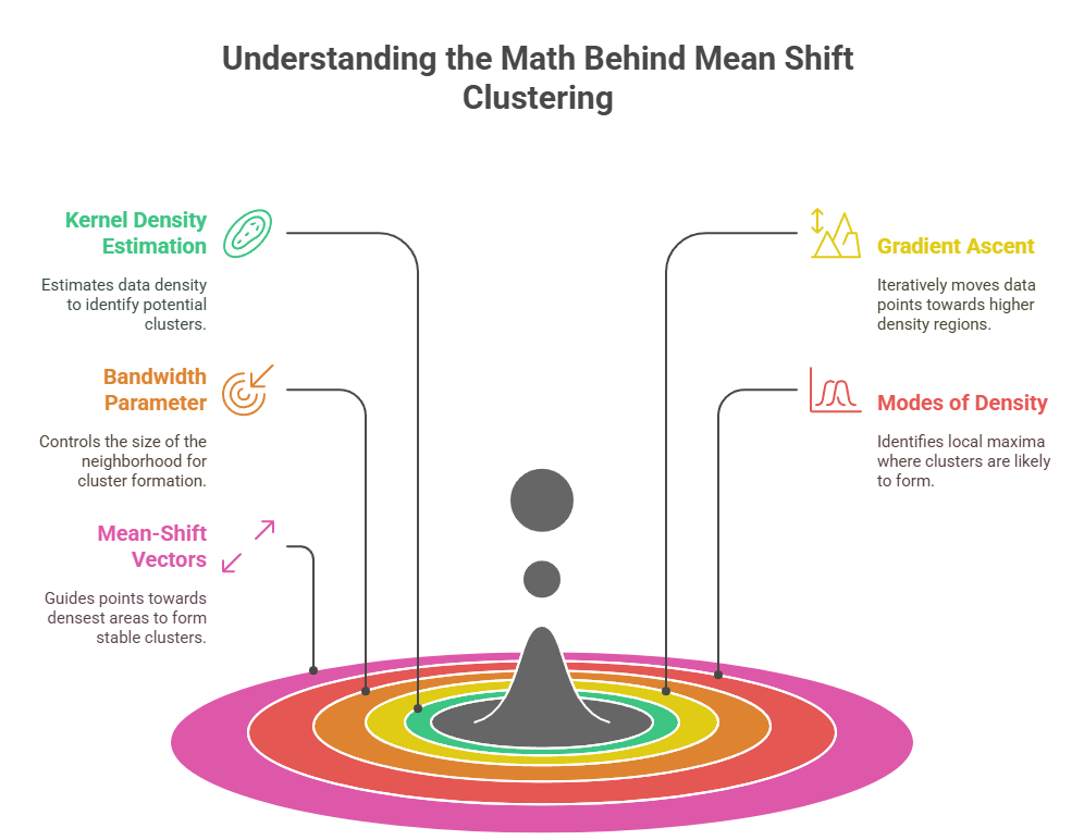
The mean shift algorithm is grounded in kernel density estimation (KDE) and gradient ascent, which helps identify clusters based on data density. Shifting data points toward the peaks of the density function iteratively refines clustering without the need for predefined cluster numbers.

Kernel Density Estimation and Gradient Ascent

Kernel Density Estimation (KDE) is a non-parametric way of estimating the probability density function of a random variable. In Mean Shift, KDE is used to estimate the density of data points in the feature space, and the algorithm works by performing gradient ascent on the density surface to find the modes (peaks of high density).

• KDE Purpose: KDE is used to estimate the data’s distribution, smoothing out the noise, and revealing underlying patterns. It allows the mean shift algorithm to understand where data points are densely grouped.
• Gradient Ascent: The mean shift algorithm performs a gradient ascent procedure where data points are shifted in the direction of the maximum increase in density. By doing this iteratively, it moves toward high-density areas or modes.
• Movement Maximizing Density: The direction of movement maximizes the local density around the data points, ensuring that the algorithm converges toward the modes of the data distribution.

Also Read: Gradient Descent in Machine Learning: How Does it Work?

Bandwidth Parameter: Role and Sensitivity

The bandwidth parameter defines the radius of influence for each point, determining how many nearby points are considered when calculating the mean. A large bandwidth smooths the data over a wider area, while a smaller bandwidth focuses on more localized neighborhoods. The choice of bandwidth has a direct impact on clustering results.

• Bandwidth as Radius: Bandwidth controls the size of the neighborhood around each point. Larger bandwidth values encompass more data points, potentially causing under-segmentation (merging distinct clusters).
• Effect of Bandwidth: Smaller bandwidth values can lead to over-segmentation (creating too many clusters), as only a small number of neighbors influence each point. The choice of bandwidth determines the granularity of the clusters formed.
• Over-Segmentation and Under-Segmentation: With a large bandwidth, the algorithm may group disparate data points together, while a small bandwidth may create clusters for each isolated point. Both scenarios can lead to inaccurate results.
• Bandwidth Selection: To determine the optimal bandwidth, methods like grid search or rule-of-thumb approaches (e.g., setting bandwidth proportional to the dataset size) can be employed. These methods help find a balance between too few and too many clusters.

How the Algorithm Finds Modes of the Density Function

In the context of Mean Shift, a "mode" refers to a local maximum in the estimated density function. The algorithm guides data points toward these modes, which are essentially the densest regions of the data, where clusters are formed.

• Mode as Local Maximum: A mode is a point where the density of neighboring data points is highest. In machine learning, these modes represent the natural groupings of data.
• Mean-Shift Vectors: The algorithm calculates mean-shift vectors, which represent the direction in which each data point moves to converge toward a mode. These vectors guide the points to the densest regions of the data.
• Density Peaks and Clusters: The final clusters formed in mean shift correspond to the local maxima of the density function, where data points have converged. These peaks represent the true structure of the data, providing more accurate clustering than methods like K-Means, which assume a fixed number of clusters.

Upgrade your skills with upGrad's Job-Linked Data Science Advanced Bootcamp. Gain practical experience through 11 live projects and become proficient in over 17 industry tools. Earn certifications from top names like Microsoft, NSDC, and Uber, and build a solid AI and machine learning portfolio that sets you apart.

Also Read: Machine Learning Tutorial: Learn ML from Scratch

Now that you've explored the mathematical intuition behind Mean Shift, let's move on to implementing it in Python for hands-on experience.

Implementing Mean Shift Clustering in Python

Implementing mean shift clustering in Python is straightforward with the scikit-learn library. This section will guide you through the necessary setup, show how to apply mean shift on a toy dataset, and visualize the clusters using matplotlib.

Key Setup and Imports:

1. Required Imports: Start by importing the necessary libraries:

from sklearn.cluster import MeanShift
from sklearn.datasets import make_blobs
import matplotlib.pyplot as plt

2. Data Format and Parameters: Mean shift requires a 2D array of features. We’ll generate synthetic data using make_blobs to create a toy dataset with multiple clusters for simplicity.

• Bandwidth: The bandwidth parameter controls the size of the neighborhood and plays a critical role in how clusters are formed. We will use the default bandwidth, but can adjust it as needed.

3. Default Settings and Configuration: The default settings for MeanShift will use a heuristic for bandwidth, and we can configure additional parameters like bin_seeding or n_jobs (for parallelization).

Common Errors:

• Shape mismatch: Ensure your input data is a 2D array.
• Choosing incorrect bandwidth: Too small or too large a bandwidth may result in overfitting or underfitting.

Running Mean Shift on a Toy Dataset

Here is a code snippet to apply mean shift on a toy dataset and visualize the clusters:

# Import necessary libraries
from sklearn.cluster import MeanShift
from sklearn.datasets import make_blobs
import matplotlib.pyplot as plt

# Generate toy data with 4 clusters
X, _ = make_blobs(n_samples=300, centers=4, cluster_std=0.60, random_state=0)

# Apply Mean Shift clustering
mean_shift = MeanShift()
mean_shift.fit(X)

# Get the cluster centers
centers = mean_shift.cluster_centers_

# Plot the data points and the cluster centers
plt.figure(figsize=(8, 6))
plt.scatter(X[:, 0], X[:, 1], c=mean_shift.labels_, cmap='viridis')
plt.scatter(centers[:, 0], centers[:, 1], s=200, c='red', marker='X')
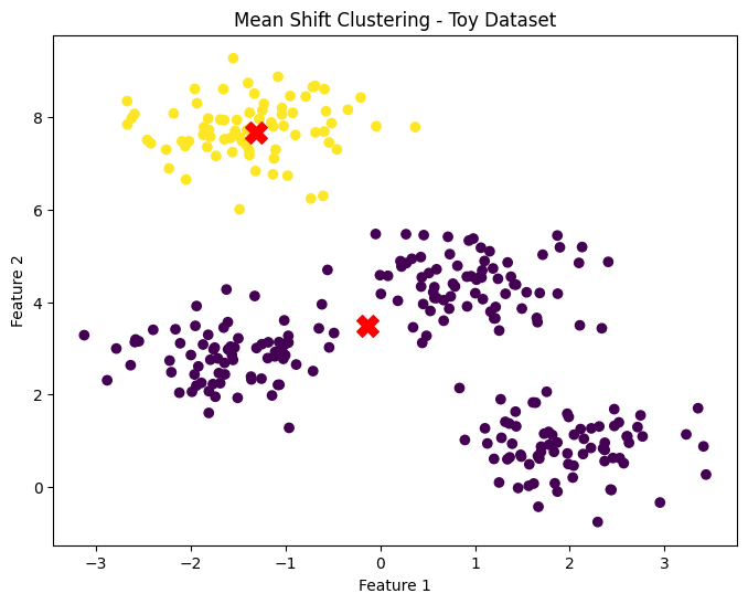
plt.title("Mean Shift Clustering - Toy Dataset")
plt.xlabel('Feature 1')
plt.ylabel('Feature 2')
plt.show()

Output:

Explanation:

• make_blobs creates a synthetic dataset with 4 clusters.
• MeanShift.fit(X) performs the clustering.
• cluster_centers_ provides the coordinates of the cluster centers.
• Matplotlib is used to plot both the data points and cluster centers, where each point is colored based on its assigned cluster.

Output Interpretation:

The plot displays the dataset with data points colored according to their cluster assignments. Red 'X' marks represent the cluster centers, showing how mean shift has grouped the data.

Common Pitfalls:

• Inconsistent Data Format: Always check the shape of your data before passing it to the fit() function.
• Bandwidth Choice: Experiment with different bandwidth values if the default does not give satisfactory results.
• Performance: On larger datasets, running the algorithm can be slow; consider using parallelization or adjusting the dataset size for testing purposes.

Implementing Mean Shift Clustering in Python

In this section, we'll extend the previous implementation of mean shift clustering to manually set the bandwidth parameter and estimate the optimal bandwidth using the estimate_bandwidth method. We will also demonstrate how tuning the bandwidth affects the cluster count and provide performance tips for handling larger datasets.

Manually Setting the Bandwidth

The bandwidth parameter controls the size of the neighborhood for each data point. A smaller bandwidth leads to many small clusters, while a larger bandwidth results in fewer larger clusters. You can manually set the bandwidth in MeanShift to see how the clusters change.

from sklearn.cluster import MeanShift
from sklearn.datasets import make_blobs
import matplotlib.pyplot as plt

# Generate toy data with 4 clusters
X, _ = make_blobs(n_samples=300, centers=4, cluster_std=0.60, random_state=0)

# Apply Mean Shift with a manually set bandwidth
mean_shift = MeanShift(bandwidth=1.5)  # manually set bandwidth
mean_shift.fit(X)

# Get the cluster centers
centers = mean_shift.cluster_centers_

# Plot the data points and the cluster centers
plt.figure(figsize=(8, 6))
plt.scatter(X[:, 0], X[:, 1], c=mean_shift.labels_, cmap='viridis')
plt.scatter(centers[:, 0], centers[:, 1], s=200, c='red', marker='X')
plt.title("Mean Shift Clustering with Manually Set Bandwidth")
plt.xlabel('Feature 1')
plt.ylabel('Feature 2')
plt.show()

Output:

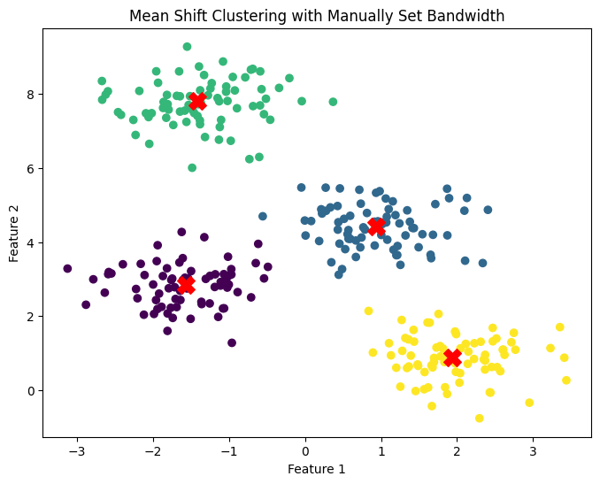
Explanation:

• The bandwidth is set to 1.5, which controls how far data points can be from the center of a cluster before being grouped into it.
• The rest of the code is similar to our previous example but includes the manual bandwidth setting.
• The resulting plot shows how clusters are formed based on the manually set bandwidth.

Output Interpretation:

• With a smaller bandwidth, you might observe more clusters. As the bandwidth increases, fewer and larger clusters will appear.

Estimating Optimal Bandwidth Using estimate_bandwidth

To find the optimal bandwidth for your dataset, scikit-learn provides a function called estimate_bandwidth. This method estimates the bandwidth based on the data's density.

from sklearn.cluster import MeanShift, estimate_bandwidth
from sklearn.datasets import make_blobs
import matplotlib.pyplot as plt

# Generate toy data with 4 clusters
X, _ = make_blobs(n_samples=300, centers=4, cluster_std=0.60, random_state=0)

# Estimate the optimal bandwidth
bandwidth = estimate_bandwidth(X, quantile=0.2, n_samples=300)

# Apply Mean Shift with estimated bandwidth
mean_shift = MeanShift(bandwidth=bandwidth)
mean_shift.fit(X)

# Get the cluster centers
centers = mean_shift.cluster_centers_

# Plot the data points and the cluster centers
plt.figure(figsize=(8, 6))
plt.scatter(X[:, 0], X[:, 1], c=mean_shift.labels_, cmap='viridis')
plt.scatter(centers[:, 0], centers[:, 1], s=200, c='red', marker='X')
plt.title("Mean Shift Clustering with Estimated Bandwidth")
plt.xlabel('Feature 1')
plt.ylabel('Feature 2')
plt.show()

Output:

Explanation:

• The estimate_bandwidth function is used to estimate the bandwidth automatically based on the dataset.
• The quantile parameter controls how aggressive the bandwidth estimation is. A lower quantile gives a larger bandwidth.
• After estimating the bandwidth, MeanShift is applied with the optimal bandwidth value.

Output Interpretation:

• The plot shows how the estimated bandwidth affects the clusters, providing a more accurate and data-driven approach than manually setting the bandwidth.

Tuning Bandwidth and Its Effect on Cluster Count

Tuning the bandwidth parameter allows you to control the number of clusters formed. A smaller bandwidth may produce more clusters, while a larger bandwidth will likely produce fewer, more generalized clusters.

# Experiment with different bandwidths and observe the effect on the number of clusters
bandwidths = [0.5, 1.0, 2.0]  # Try different bandwidth values
for bandwidth in bandwidths:
    mean_shift = MeanShift(bandwidth=bandwidth)
    mean_shift.fit(X)
    
    # Plot the clusters
    plt.figure(figsize=(8, 6))
    plt.scatter(X[:, 0], X[:, 1], c=mean_shift.labels_, cmap='viridis')
    plt.scatter(mean_shift.cluster_centers_[:, 0], mean_shift.cluster_centers_[:, 1], s=200, c='red', marker='X')
    plt.title(f"Mean Shift Clustering with Bandwidth {bandwidth}")
    plt.xlabel('Feature 1')
    plt.ylabel('Feature 2')
    plt.show()

Output:

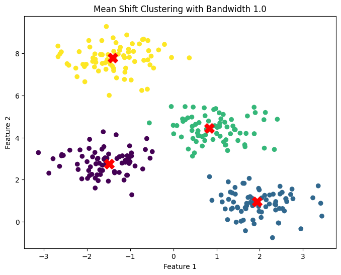
Explanation:

• We experiment with three different bandwidth values and visualize how they affect the clusters.
• The clustering results are plotted for each bandwidth, showing the impact of the bandwidth on the number of clusters.

Output Interpretation:

• As the bandwidth increases, the clusters become fewer and larger, while smaller bandwidth values create more and smaller clusters.

Performance Tips for Large Datasets

When dealing with large datasets, mean shift clustering can become computationally expensive. Here are some tips for handling large datasets more efficiently:

• Reduce Dimensionality: Use techniques like Principal Component Analysis (PCA) to reduce the feature space before applying Mean Shift.
• Use Parallelization: Use joblib or Dato to parallelize the algorithm and speed up the clustering process.
• Sampling: If your dataset is extremely large, consider using a subset of the data for initial experimentation to reduce computational time.

Ready to take your career to the next level? The Executive Diploma in Data Science & AI with IIIT-B offers a cutting-edge curriculum, hands-on experience, and mentorship from industry leaders. With 30k+ successful alumni and real-world case studies, you’ll gain expertise in Cloud Computing, Big Data, Deep Learning, Gen AI, and more in just 11 months. Secure your spot today and join the next generation of AI professionals!

Also Read: Top 29 Image Processing Projects in 2025 For All Levels + Source Code

After learning to implement mean shift clustering in Python, it's time to explore its real-world applications across various machine learning domains.

Applications of Mean Shift Clustering in Machine Learning

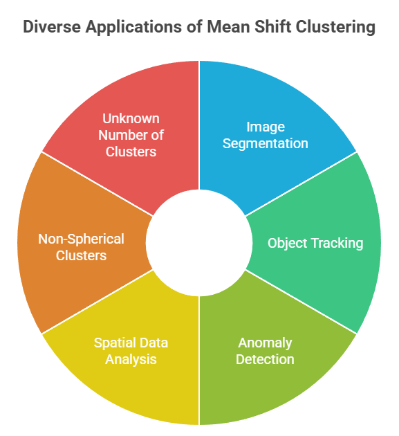
Mean shift clustering is a powerful and flexible algorithm used in various machine learning applications, particularly in scenarios where traditional clustering methods like K-Means may fall short. Below are some key areas where mean shift clustering has proven to be effective:

1. Image Segmentation and Object Tracking

Mean shift clustering excels in segmenting images and tracking objects across frames, particularly in computer vision tasks. It identifies regions of high-density pixels and can adapt to the natural distribution of the data, which is crucial for segmenting complex or irregular shapes in images.

• Image Segmentation: It divides images into meaningful regions by grouping similar pixels, useful in medical imaging and autonomous vehicles for detecting boundaries.
• Object Tracking: In dynamic environments, mean shift tracks the movement of objects in videos. By detecting high-density regions, it can follow objects across frames, such as tracking a car on a road in real-time.

Also read: Image Recognition Machine Learning: Brief Introduction

2. Anomaly Detection and Spatial Data Analysis

Mean shift is widely applied in anomaly detection, especially in spatial data, where patterns of density can reveal outliers or unusual events.

• Anomaly Detection: The algorithm detects regions with low data density, which can indicate outliers or anomalies. In fraud detection and network security, for instance, isolated modes or low-density convergence points are interpreted as anomalies, suggesting unusual or suspicious activities, such as fraudulent transactions or unauthorized access. This method is also useful in identifying rare events in time-series data, where anomalies deviate from the expected patterns.
• Spatial Data Analysis: Mean shift is used to analyze geographical or spatial data, such as customer locations, weather patterns, or real estate pricing, by finding dense clusters or unusual regions of data. By identifying areas of high concentration, it helps reveal significant trends while also detecting anomalous regions with low density that may indicate emerging patterns or outliers.

Also Read: Understanding the Role of Anomaly Detection in Data Mining

Use Cases Where K-Means Fails but Mean Shift Works

While K-Means is a widely used clustering method, it struggles with datasets where clusters have non-spherical shapes or when the number of clusters is unknown. Mean shift overcomes these limitations with its flexibility.

• Non-Spherical Clusters: K-Means assumes spherical clusters, which limits its ability to identify clusters with arbitrary shapes. Mean shift adapts to the data's natural distribution and finds clusters of any shape, making it ideal for complex datasets.
• Unknown Number of Clusters: Unlike K-Means, which requires pre-defining the number of clusters, Mean shift automatically identifies the number of clusters based on data density. This is especially useful in exploratory data analysis where the true cluster structure is unknown.

Key Use Cases

• Autonomous Vehicles: Mean shift is used for object tracking and segmentation in autonomous vehicles, such as detecting road signs, pedestrians, and other vehicles. It helps in accurately identifying and tracking these objects in dynamic environments.
• Medical Imaging: Segmenting different regions in scans or images, such as identifying tumors in X-ray or MRI images.
• Geospatial Analysis: Mean shift is highly effective in geospatial analysis, detecting regions of interest like urban areas or forest clusters from satellite imagery. Identifying areas of high data density distinguishes between populated urban regions and less-dense rural or forested areas. This makes it valuable for environmental monitoring, urban planning, and land-use analysis.

Looking to boost your career in AI and Data Science? The 1-Year Master's Degree in AI & Data Science from O.P. Jindal Global University offers 15+ projects, 500+ hours of learning, and Microsoft Certification. Master tools like Python and Power BI, plus get free access to Microsoft Copilot Pro. Apply now and advance in just 12 months!

Also Read: Top 5 Machine Learning Models Explained For Beginners 

Having explored the diverse applications of mean shift clustering, it's time to examine the advantages and limitations of this algorithm.

Pros and Cons of the Mean Shift Algorithm

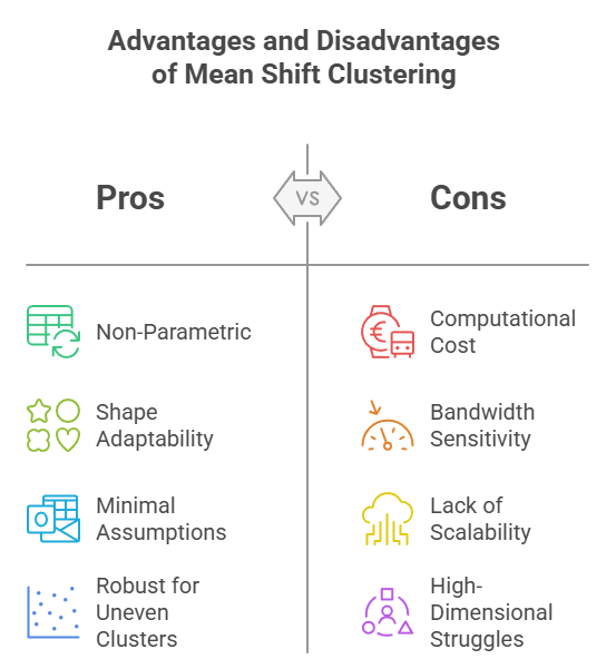
Mean shift clustering offers several advantages for clustering tasks, but it also comes with a set of limitations. It’s essential to weigh these factors when deciding whether to use this algorithm, depending on your dataset's characteristics and the problem.

Benefits: Flexibility, No K Needed, Shape Adaptability

Mean shift is valued for its ability to handle diverse clustering challenges without defining the number of clusters in advance.

• Non-Parametric and Flexible: Mean shift does not require a predefined number of clusters, allowing it to naturally adapt to the distribution of data. This makes it ideal when the number of clusters is unknown or uncertain.
• Shape Adaptability: Unlike K-Means, which assumes spherical clusters, mean shift can identify clusters of any shape. This is particularly useful when clusters vary in density or have irregular, elongated forms, ensuring greater precision.
• Minimal Assumptions About the Data: The algorithm makes very few assumptions about the data, allowing for easy implementation and reducing model bias. This simplicity makes it highly adaptable to various data types.
• Robustness for Uneven and Overlapping Clusters: Mean shift excels when dealing with clusters with uneven densities or overlap, which can be problematic for algorithms like K-Means. This ensures more accurate results with complex datasets.

Limitations: Computational Cost and Bandwidth Sensitivity

Despite its strengths, mean shift has several drawbacks that should be considered, especially when dealing with large or complex datasets.

• Computational Cost: The iterative process used by mean shift to shift data points towards modes can be computationally expensive. This becomes more pronounced with large datasets, where significant processing power is required. Solution: To mitigate this, techniques like down-sampling, parallel computing, or approximations such as the fast mean shift algorithm can be applied to improve efficiency.
• Bandwidth Sensitivity: The performance of mean shift is highly sensitive to the bandwidth parameter. Choosing the wrong bandwidth can lead to poor results—overfitting with a too-small bandwidth or underfitting with too large a bandwidth. Solution: Cross-validation or methods like the Silverman method can help in selecting the optimal bandwidth for more stable results.
• Lack of Scalability: While mean shift performs well with smaller datasets, it struggles with large-scale data. As dataset sizes increase, the computational cost and time required for convergence become prohibitive. Solution: Using parallel computing or distributed computing frameworks like Hadoop or Spark can alleviate scalability issues by splitting the computation across multiple nodes.
• Poor Performance on High-Dimensional Data:In high-dimensional spaces, the concept of density becomes less meaningful. The "curse of dimensionality" causes data to become sparse, making local density estimates unreliable. This can hinder Mean Shift’s ability to detect meaningful clusters. As dimensionality increases, the algorithm becomes slower and less effective. 

Solution: Dimensionality reduction techniques like PCA (Principal Component Analysis) can be applied before running mean shift to reduce the number of dimensions and improve its performance.

Also read: What is Overfitting & Underfitting In Machine Learning? [Everything You Need to Learn]

When to Prefer Mean Shift Over Other Algorithms?

Mean shift excels in specific use cases, but it's essential to consider when it is the most suitable choice based on your data and requirements.

• Small-to-Medium Datasets with Unknown K: When you don’t have a predefined number of clusters (K), mean shift is an ideal solution because it automatically determines the number of clusters based on the data’s density, making it particularly useful for exploratory data analysis.
• Unknown or Non-Spherical Clusters: Mean shift is the better choice when the clusters have irregular shapes or varying densities, which traditional algorithms like K-Means can struggle with. This allows for more accurate grouping in datasets with complex, non-linear structures.
• Avoid for Huge Datasets: For large datasets where computational efficiency is a priority, mean shift may not be the best option. Algorithms like K-Means or MiniBatchKMeans are more scalable and faster for extensive data.
• Comparison with DBSCAN and Hierarchical Clustering: Mean shift is similar to DBSCAN in that both are density-based, but mean shift is more flexible with cluster shapes and can be more intuitive for understanding data distributions. Compared to hierarchical clustering, mean shift can be more scalable and faster, although hierarchical clustering provides better insight into the cluster hierarchy.

Also Read: Types of Machine Learning Algorithms with Use Cases Examples

Now that you understand when mean shift is the best option, it's time to put your knowledge to the test with some practical questions.

Test Your Expertise in Mean Shift Clustering

Test your understanding of mean shift Clustering with these multiple-choice questions:

1. What does the mean shift algorithm rely on to find clusters?
2. • A) K predefined clusters
   • B) Density peaks
   • C) Cluster Centers
   • D) Grid search
2. Which of the following is an advantage of mean shift over K-Means?
3. • A) It requires a predefined K
   • B) It can handle irregularly shaped clusters
   • C) It is faster on large datasets
   • D) It only works with numerical data
3. What parameter in the mean shift algorithm controls the neighborhood size?
4. • A) Number of iterations
   • B) Bandwidth
   • C) K value
   • D) Cluster radius
4. What is the primary reason that K-Means can struggle with complex datasets?
5. • A) It requires dense data
   • B) It assumes spherical clusters
   • C) It uses density peaks
   • D) It is computationally inefficient
5. Which of the following is NOT a typical application of mean shift clustering?
6. • A) Image segmentation
   • B) Customer segmentation
   • C) Text generation
   • D) Anomaly detection
6. How does mean shift determine the number of clusters?
7. • A) By using a fixed number of clusters
   • B) By iterating and finding density peaks
   • C) By using user-provided labels
   • D) By splitting data into equal-sized groups
7. What is a key disadvantage of mean shift when working with high-dimensional data?
8. • A) It does not scale well
   • B) It struggles with sparse data
   • C) It assumes spherical clusters
   • D) It requires labeled data
8. Which of these clustering algorithms is density-based, like Mean Shift?
9. • A) K-Means
   • B) DBSCAN
   • C) Linear Regression
   • D) PCA
9. Which of the following is a common issue when using mean shift with large datasets?
10. • A) Slow convergence
    • B) Inability to detect clusters
    • C) Overfitting
    • D) Uncertainty in clustering
10. What is the bandwidth parameter on the mean shift algorithm?
11. • A) The shape of the data
    • B) The number of data points to process
    • C) The size of the neighborhood for each point
    • D) The number of iterations needed

Now that you've tested your understanding of mean shift Clustering, it's time to take your knowledge to the next level.

Master Mean Shift Clustering and Machine Learning with upGrad

Mean shift clustering is a versatile technique that excels in handling complex, non-linear data distributions. Unlike traditional methods like K-Means, it doesn’t require predefined cluster numbers, making it perfect for exploratory data analysis. However, managing the algorithm's computational costs and bandwidth sensitivity is essential for optimal results.

If you're eager to master advanced machine learning methods such as Mean Shift, upGrad's in-depth AI and machine learning courses provide expert-led instruction, equipping you with the skills to apply these techniques to real-world data science projects.

Here are some of the top courses to help you level up your machine learning expertise:

• Master's Degree in Artificial Intelligence and Data Science
• Master's in Data Science Degree

You can also check out these additional free courses to enhance your learning:

• Artificial Intelligence in the Real World
• Introduction to Natural Language Processing

Not sure which program aligns best with your career objectives?

upGrad offers personalized one-on-one career counseling to help you choose the right learning path based on your goals and experience. You can also visit any upGrad centre for hands-on training with experienced mentors.   

FAQs

1. How does Mean Shift clustering identify cluster centers differently from centroid-based methods?

Unlike centroid-based methods that assign cluster centers arbitrarily or based on initial guesses, Mean Shift identifies cluster centers by moving data points iteratively toward the nearest high-density region, effectively locating true modes of the data distribution. This approach allows cluster centers to emerge naturally from the data without relying on assumptions about cluster shapes or numbers. Consequently, the resulting clusters better represent the inherent structure of complex datasets.

2. How does the choice of kernel affect Mean Shift clustering results?

The kernel function defines the weighting of points within the neighborhood and impacts the smoothness of density estimation. Common kernels include Gaussian and Epanechnikov. A Gaussian kernel provides smooth weighting decreasing with distance, making it well-suited for continuous data, while other kernels may offer sharper boundaries. Choosing the right kernel can affect cluster shape sensitivity and convergence speed. Selecting an inappropriate kernel can lead to either overly smooth clusters or excessive fragmentation.

3. What computational challenges arise when applying Mean Shift clustering?

Since Mean Shift iteratively calculates the weighted mean of points in local neighborhoods for every data point, it can be computationally expensive, especially for large datasets or high dimensions. This repeated neighborhood search and mean calculation lead to slow runtimes. Efficient implementations often use techniques like KD-trees or approximate nearest neighbors to reduce this overhead. Without such optimizations, running Mean Shift on very large datasets may become impractical.

4. Can Mean Shift clustering be parallelized or optimized for big data?

Yes, the iterative nature of Mean Shift allows for parallelization since the shifts of individual points are independent in each iteration. Frameworks that support parallel computation or GPU acceleration can speed up clustering. Additionally, data sampling, approximate neighbor search, and dimensionality reduction can help scale Mean Shift to larger datasets while maintaining reasonable accuracy. These approaches help extend Mean Shift’s usability beyond small to medium-sized datasets.

5. How does Mean Shift clustering handle overlapping clusters or clusters with varying densities?

Because it is based on density peaks, Mean Shift naturally adapts to clusters with different densities and can separate overlapping clusters as long as they correspond to distinct modes in the density function. This is an advantage over algorithms like K-Means, which may merge such clusters due to reliance on distance to centroids. Consequently, Mean Shift often produces more meaningful clusters in real-world data where overlaps and density variations are common.

6. How important is the initial position of data points in Mean Shift clustering?

Unlike algorithms that depend on initial centroids, Mean Shift treats every data point as a candidate for shifting towards a mode, which reduces sensitivity to initialization. This approach allows the algorithm to explore the density surface more thoroughly, increasing robustness and reducing the risk of converging to poor local minima. Therefore, it generally offers more stable and consistent clustering outcomes across runs.

7. What types of datasets or problems are unsuitable for Mean Shift clustering?

Datasets with extremely high dimensionality, very large size without dimensionality reduction, or data where density is not a meaningful concept (e.g., categorical data without proper encoding) may challenge Mean Shift. Additionally, datasets where clusters are defined more by proximity or connectivity than density may be better served by alternative methods. In such cases, methods tailored for sparse or categorical data could provide better results.

8. How does Mean Shift clustering deal with noise and outliers?

Noise points generally reside in low-density areas and fail to form modes during the iterative shifting process. As a result, Mean Shift effectively ignores these points or treats them as separate minor clusters that can be filtered out. This robustness to noise makes it suitable for real-world noisy data. However, extreme outliers far from any dense region may still require pre-processing or additional filtering.

9. What role does convergence criteria play in the quality of Mean Shift clustering?

The convergence threshold determines when the iterative shifting stops—usually when shifts between iterations fall below a small value. Setting this threshold too high can result in premature stopping and inaccurate clusters, while too low a threshold may cause unnecessary computation. Proper tuning ensures clusters are stable and representative of true density modes. Fine-tuning convergence criteria can also impact runtime efficiency.

10. How does Mean Shift clustering integrate with other machine learning workflows?

Mean Shift can serve as a preprocessing step for feature engineering by identifying natural groupings in data. It can also be combined with classification or anomaly detection systems to label data points or detect outliers. Additionally, in computer vision, it’s often paired with tracking or segmentation models to refine object boundaries dynamically. This versatility allows it to be a valuable component across diverse ML pipelines.

11. Are there any common heuristics or rules of thumb for setting Mean Shift parameters?

Beyond bandwidth, practitioners often use heuristic methods such as setting bandwidth proportional to the data’s standard deviation or employing cross-validation to balance cluster granularity. Visual inspection of clustering results at different bandwidths and kernels is also a practical way to select parameters that align with domain-specific patterns. Experimentation remains key since optimal settings can vary significantly by dataset.