CNN Architecture: Components, Working, Popular Models, and Real-World Applications

Quick Overview of CNN Architecture

• CNN (Convolutional Neural Network) architecture is a deep learning model designed to process and understand images.
• It uses layers such as convolution, activation, pooling, and fully connected layers to automatically learn features and make predictions.
• CNNs are widely used for image classification, object detection, image recognition, facial recognition, and other computer vision tasks.
• Popular CNN architectures include LeNet, AlexNet, VGG, ResNet, and EfficientNet.
• The right CNN architecture depends on the problem, dataset, and performance requirements.

In this guide, you'll learn about the architecture of CNN, how it works, the purpose of each layer, and the mathematics behind convolution in a simple way. We'll also explore popular CNN architectures, compare CNNs with other deep learning models, and understand their real-world applications.

Interested in learning how CNNs fit into the broader field of AI? Our Artificial Intelligence Course covers deep learning, computer vision, neural networks, and real-world AI applications to help you build job-ready skills.

What is CNN Architecture?

A Convolutional Neural Network (CNN) is a type of deep learning model designed to process and understand visual data such as images and videos.

Unlike traditional neural networks that process every input independently, CNNs analyze small regions of an image to identify patterns like edges, textures, and shapes. This makes them highly effective for computer vision tasks such as image classification, object detection, and image recognition.

CNN architecture refers to the arrangement of different layers that work together to extract features from an image and make predictions.

As an image passes through these layers, the network gradually learns simple features in the initial stages and more complex patterns in the deeper layers, enabling it to accurately identify and classify objects.

Components of CNN Architecture

A basic CNN architecture consists of 6 layers, each designed to perform a specific task. These layers work together to transform a raw image into meaningful features and finally produce a prediction. While the input layer receives the image, the intermediate layers extract and refine visual features, and the final layers use those features to classify the image.

In this section, we will explore different components of the CNN architecture and the mathematics behind it.

1. Input Layer

The Input Layer is the first layer of a CNN and serves as the entry point for the input image. Unlike humans, a CNN cannot interpret an image directly. Instead, it receives the image as a collection of numerical pixel values.

For a grayscale image, each pixel has a single intensity value ranging from 0 (black) to 255 (white).

For a color image, each pixel is represented using three color channels:

• Red (R)
• Green (G)
• Blue (B)

These three channels together form an RGB image.

For example, if an image has a resolution of 224 × 224 pixels, its input size becomes:

Input Shape = Height × Width × Channels

Input Shape = 224 × 224 × 3

where:

• 224 = Height of the image
• 224 = Width of the image
• 3 = RGB color channels

This means the CNN receives a three-dimensional matrix (also called a tensor) containing the pixel values of the image.

2. Convolutional Layer in CNN Architecture

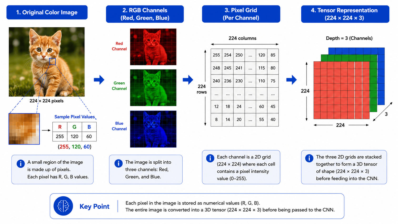
The Convolution Layer is the most important component of a CNN. Its job is to scan the input image and identify useful visual features such as edges, corners, textures, and patterns.

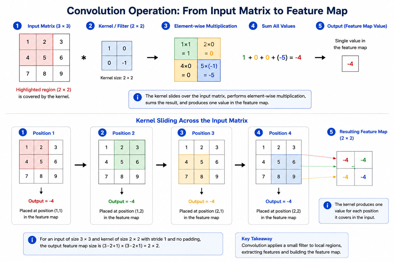
Instead of processing the entire image at once, the convolution layer uses a small matrix called a filter (or kernel) that moves across the image one region at a time. At each position, the filter performs a mathematical operation called the dot product between the filter values and the corresponding pixel values.

The result of this operation is stored in a new matrix called the feature map. By applying multiple filters, the CNN can learn different types of visual features from the same image.

Mathematical Representation of Convolutional Operation

The convolution operation can be expressed as:

Where:

• Input = Original image
• Kernel = Small filter used to detect features
• Output = Feature map
• (i, j) = Current position of the filter

In simple terms, the CNN multiplies the values of the filter with the corresponding pixel values, adds the results together, and stores the final value in the feature map.

Simple Example

Suppose the input image is:

1	2	3
4	5	6
7	8	9

and the filter is:

1	0
0	-1

The first convolution operation is:

(1×1) +(2×0) + (4×0) + (5×-1) = 1 - 5 = -4 

The value -4 becomes the first element of the feature map.

The filter then moves to the next region and repeats the same process until the complete feature map is generated.

3. Activation Function (ReLU)

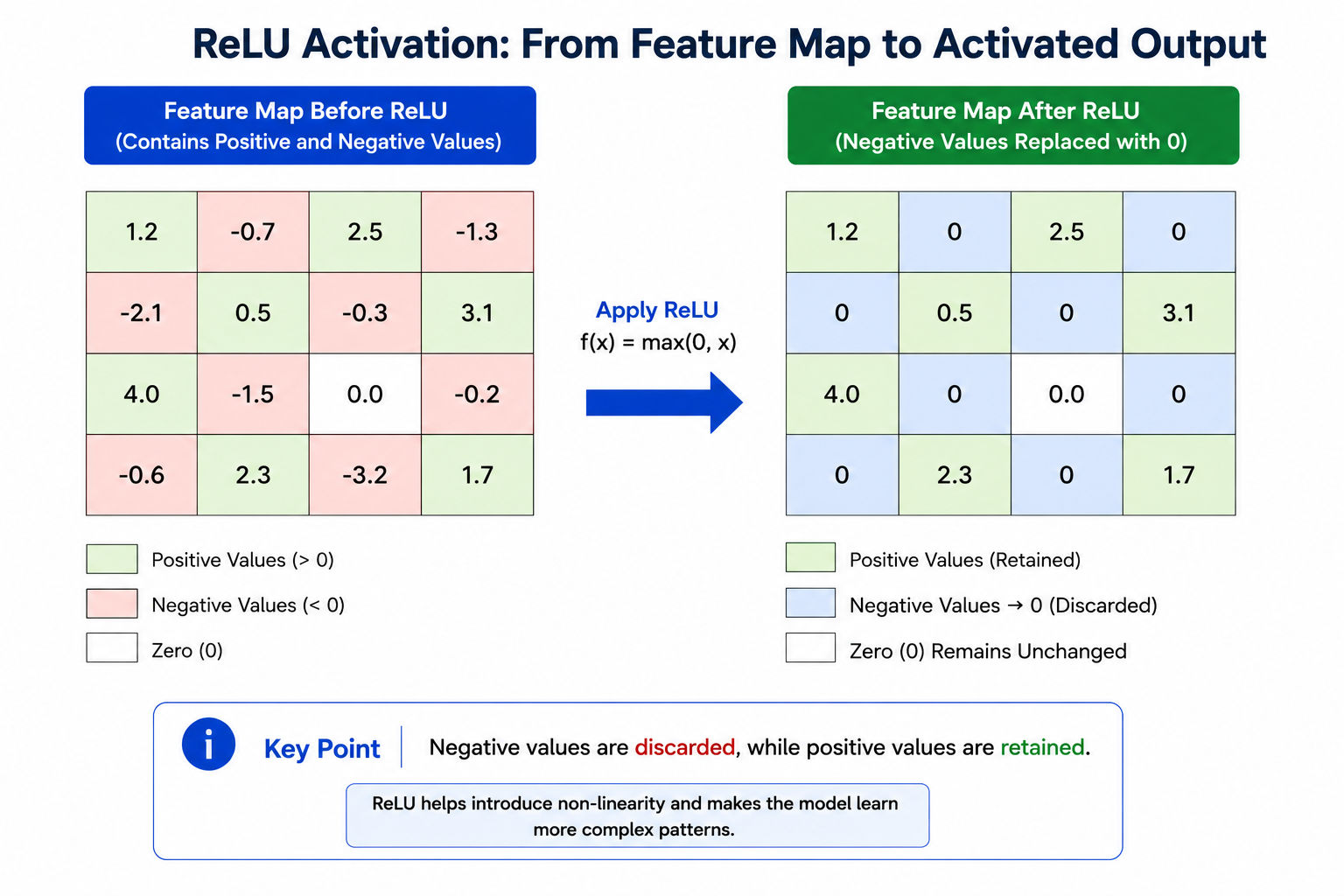
After the convolution operation, the feature map passes through an activation function. Its purpose is to help the CNN learn complex patterns that cannot be captured using only linear mathematical operations.

The most commonly used activation function is the Rectified Linear Unit (ReLU).

Mathematical Formula of ReLU Activation Function

ReLU(x) = max(0, x)

This means:

• If the value is positive, it remains unchanged.
• If the value is negative, it becomes 0.

Example

You Can Also Explore: Math for Machine Learning: Essential Concepts You Must Know

4. Pooling Layer

As the image passes through multiple convolution layers, the generated feature maps become larger and contain a significant amount of information. Processing these large feature maps increases the computational cost and may also lead to overfitting, where the model performs well on training data but poorly on new data.

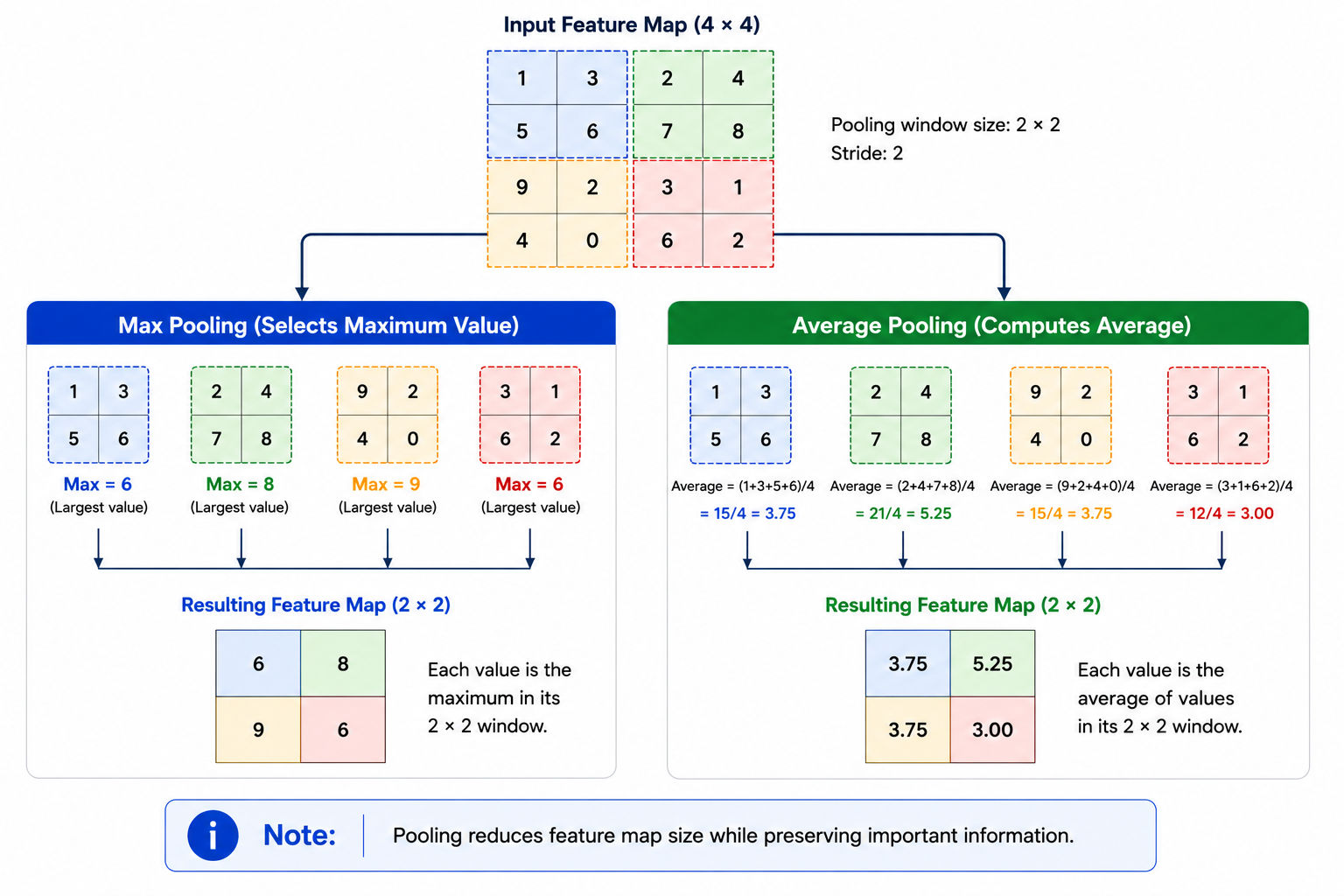
The Pooling Layer in CNN architecture solves this problem by reducing the size of the feature maps while preserving the most important features. This process is called down sampling and helps the CNN become faster, more memory-efficient, and better at generalizing to unseen images.

The two most commonly used pooling techniques are:

• Max Pooling: Selects the largest value from a small region.
• Average Pooling: Calculates the average value of all elements in a small region.

5. Fully Connected Layer

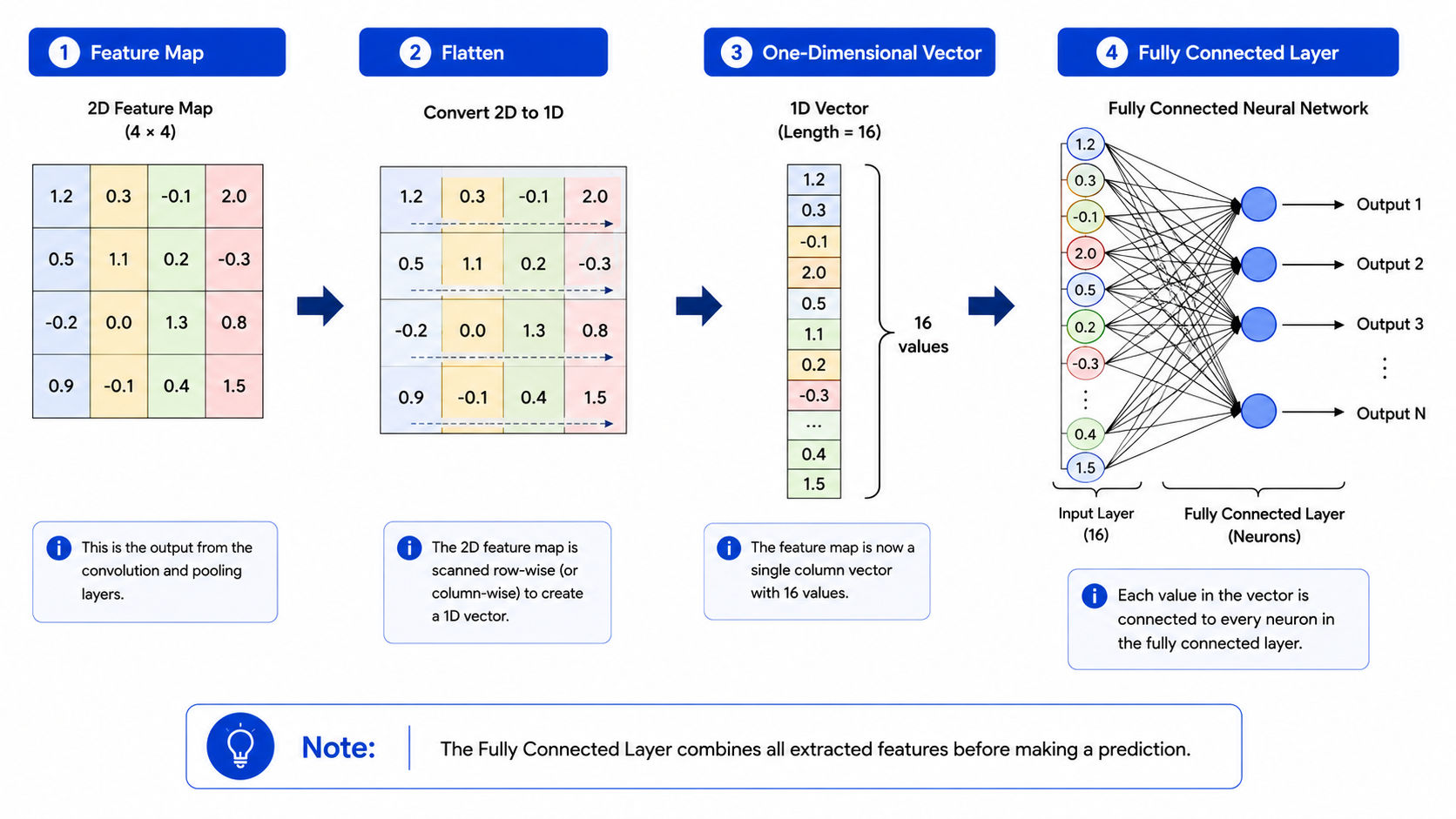
After the convolution and pooling layers have extracted the important features, the CNN must use these features to make a prediction. This is the role of the Fully Connected Layer in CNN.

Before entering the Fully Connected Layer, the feature maps are converted into a one-dimensional vector through a process called Flattening.

Example: 

6. Output Layer

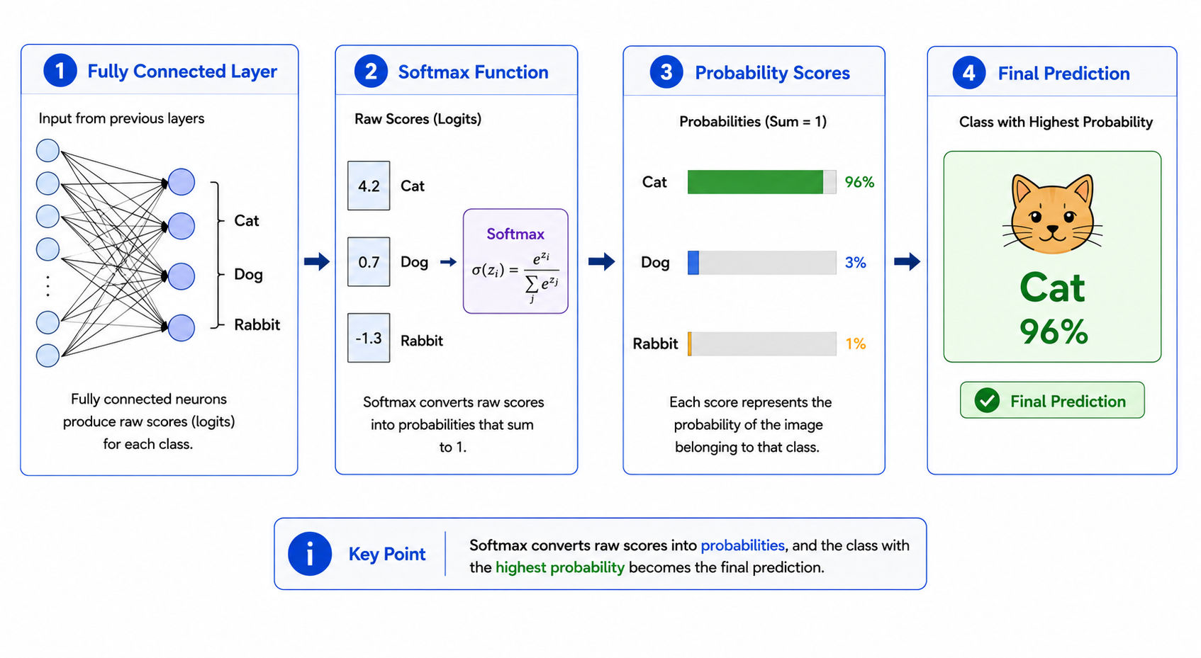
The Output Layer is the final layer of a CNN. It receives the scores generated by the Fully Connected Layer and converts them into probabilities for each possible class.

For multi-class image classification, CNNs commonly use the Softmax activation function.

Mathematical Formula

Where:

• zi = Score assigned to class i
• P(yi) = Probability of class i
• The probabilities of all classes always add up to 1 (or 100%).

Example

Suppose the Fully Connected Layer produces the following scores:

Ready to apply concepts like CNNs to real-world AI projects? Our Diploma in Machine Learning & AI with MLOps, GenAI & Agentic AI covers everything from AI fundamentals and deep learning to modern GenAI, agentic AI, and production deployment.

How Does the Architecture of CNN Works?

A CNN processes an image in a series of steps, with each layer performing a specific task. Instead of trying to recognize an entire object at once, the network first identifies simple patterns such as edges and textures. These patterns are then combined to recognize more complex shapes and, finally, complete objects.

The following steps explain how the architecture of CNN transforms a raw image into a prediction.

Step 1: Input Image

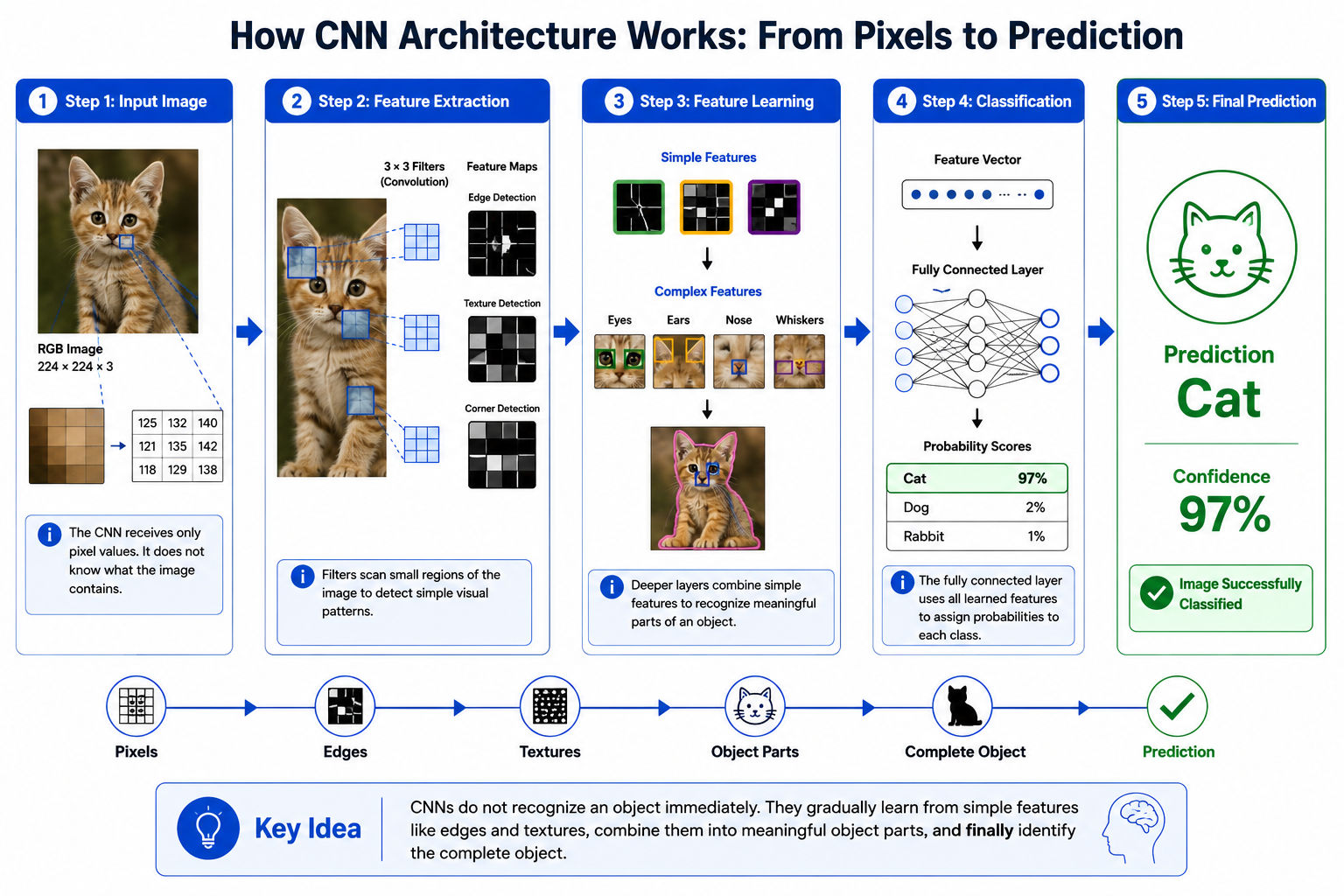
The process begins with an input image, which is represented as a grid of pixel values. For a color image, each pixel contains information for the Red (R), Green (G), and Blue (B) color channels.

At this stage, the CNN does not know what the image contains. It only receives numerical pixel values as input and uses them to learn meaningful patterns during training.

Step 2: Feature Extraction

Next, the image passes through one or more convolution layers, where the CNN begins extracting useful features. Instead of processing the entire image at once, it scans small regions using filters to detect simple patterns.

In the early layers, the CNN learns basic features such as:

• Edges
• Corners
• Lines
• Simple textures

These features form the foundation for recognizing more complex objects in later stages of the network.

Want to know more about feature extraction? Explore our blog – Feature Extraction in Machine Learning

Step 3: Feature Learning

As the image moves deeper into the network, the CNN combines the simple features learned earlier to identify more meaningful patterns.

For example, after detecting edges and curves, the network may recognize:

• Eyes
• Ears
• Wheels
• Windows
• Leaves

With additional layers, these features are combined to identify complete objects such as a cat, a car, or a tree. This hierarchical learning process enables CNNs to understand complex visual information without requiring manually defined features.

Step 4: Classification

After learning the important features, the CNN converts them into a format that can be used for prediction. These features are passed to the fully connected layer, which analyzes the extracted information and assigns probabilities to the possible classes.

The class with the highest probability becomes the model's final prediction. For example, if the network is classifying animals, the output could be:

• Cat - 97%
• Dog - 2%
• Rabbit - 1%

Since Cat has the highest probability, the CNN predicts that the image contains a cat.

Also Read - What is Classification in Machine Learning?

Popular CNN Architectures Explained

A single CNN architecture cannot solve every computer vision problem efficiently. As image datasets became larger and recognition tasks grew more complex, the limitations of early CNN models became more apparent.

To address these challenges, researchers developed new CNN architectures that improved accuracy, reduced computational cost, enabled deeper networks, and solved problems such as vanishing gradients and overfitting.

Each new architecture builds on the strengths of its predecessors while introducing innovative techniques to improve performance. 

Let's explore some of the most influential CNN architectures and understand what makes each one unique.

1. LeNet

Introduced by Yann LeCun in 1998, LeNet-5 is considered one of the earliest successful CNN architectures. It was originally developed to recognize handwritten digits for bank cheque processing and postal code recognition.

LeNet consists of a simple architecture with convolution layers, pooling layers, and fully connected layers. Although it is relatively small compared to modern CNNs, it demonstrated that neural networks could automatically learn image features without manual feature engineering.

Key Highlights of LeNet

• Introduced in 1998
• Designed for handwritten digit recognition
• One of the first successful CNN architectures
• Simple and lightweight architecture

LeNet is Best Used For

• Learning CNN fundamentals
• Small image datasets
• Educational purposes

2. AlexNet

Developed by Alex Krizhevsky, Ilya Sutskever, and Geoffrey Hinton, AlexNet won the ImageNet Large Scale Visual Recognition Challenge (ILSVRC) in 2012 and demonstrated the power of deep learning for image classification.

Compared to LeNet, AlexNet introduced a much deeper network with eight learnable layers, ReLU activation, Dropout, and GPU-based training, significantly improving both speed and accuracy.

Its success sparked widespread interest in deep learning and accelerated research in computer vision.

Key Highlights of AlexNet

• Winner of ImageNet 2012
• Introduced ReLU activation for faster training
• Used Dropout to reduce overfitting
• Trained efficiently using GPUs

AlexNet is Best Used For

• Large-scale image classification
• Learning modern CNN concepts
• Academic research

3. VGG

Developed by researchers at the University of Oxford in 2014, VGG demonstrated that increasing network depth using small 3 × 3 convolution filters could significantly improve image classification performance.

Unlike earlier architectures that used different filter sizes, VGG relied on a consistent design with repeated convolution blocks, making it simple to understand and implement.

However, its large number of parameters also made it computationally expensive.

Key Highlights of VGG

• Introduced in 2014
• Uses only 3 × 3 convolution filters
• Simple and uniform architecture
• High accuracy but computationally intensive

VGG is Best Used For

• Feature extraction
• Transfer learning
• Computer vision Research

4. ResNet

As CNNs became deeper, they faced a problem known as the vanishing gradient, where training became difficult and accuracy stopped improving. ResNet (Residual Network), introduced by Microsoft Research in 2015, solved this issue using skip connections, also known as residual connections.

Instead of learning direct mapping, ResNet allows information to bypass certain layers, making it possible to train networks with 50, 101, or even 152 layers effectively.

Today, ResNet remains one of the most widely used CNN architectures for image recognition and transfer learning.

Key Highlights of ResNet

• Introduced in 2015
• Uses residual (skip) connections
• Solves the vanishing gradient problem
• Enables training of very deep networks

ResNet is Best Used For

• Image classification
• Object detection
• Transfer learning

5. DenseNet

DenseNet (Densely Connected Convolutional Network) was introduced in 2017 to improve information flow within deep neural networks. Instead of connecting only adjacent layers, DenseNet connects every layer to all subsequent layers.

This dense connectivity encourages feature reuse, improves gradient flow, and reduces the number of parameters compared to similarly deep networks.

As a result, DenseNet achieves high accuracy while remaining computationally efficient.

Key Highlights of DenseNet

• Introduced in 2017
• Dense connections between layers
• Encourages feature reuse
• Fewer parameters than many deep CNNs

DenseNet is Best Used For

• Medical image analysis
• Image classification
• Resource-efficient deep learning

6. EfficientNet

Introduced by Google Research in 2019, EfficientNet addressed a common challenge in CNN design: how to improve accuracy without significantly increasing computational cost.

Previous architectures often became better by simply adding more layers or using larger images. EfficientNet introduced compound scaling, which balances the network's depth, width, and input image resolution simultaneously. This allows it to achieve high accuracy while using fewer parameters and less computational power.

Today, EfficientNet is widely used in real-world applications where both performance and efficiency are important.

Key Highlights of EfficientNet

• Introduced in 2019
• Uses compound scaling
• High accuracy with fewer parameters
• Optimized for speed and efficiency

EfficientNet is Best Used For

• Mobile and edge AI applications
• Image classification
• Real-time computer vision

Application of CNN Architecture

CNN architecture has transformed the way computers analyze and understand visual information. By automatically learning features from images, CNNs can perform tasks that would otherwise require extensive manual analysis. 

Today, CNNs are used across industries to improve accuracy, reduce manual effort, and automate image-based decision-making. Let's explore some of the most common applications of CNN architecture.

1. Medical Imaging

What is it?

Medical imaging involves analyzing images such as X-rays, CT scans, MRI scans, and ultrasound images to identify diseases and abnormalities.

How does CNN help?

CNNs automatically learn patterns from medical images and can detect abnormalities such as tumors, fractures, or lung infections by identifying subtle visual features that may be difficult to notice.

Why is CNN used?

Medical images contain complex patterns that require accurate analysis. CNNs can process thousands of images consistently and assist doctors by highlighting suspicious regions, reducing diagnosis time and improving accuracy.

Examples

• Detecting breast cancer from mammograms
• Identifying pneumonia from chest X-rays
• Brain tumor detection using MRI scans
• Diabetic retinopathy detection from retinal images

2. Autonomous Vehicles

What is it?

Autonomous vehicles use cameras and sensors to understand their surroundings and make driving decisions.

How does CNN help?

CNNs process images captured by onboard cameras to identify roads, traffic signs, pedestrians, vehicles, cyclists, and lane markings in real time.

Why is CNN used?

Safe driving requires recognizing multiple objects simultaneously and making decisions within milliseconds. CNNs can extract visual information quickly and accurately, making them suitable for real-time navigation.

Examples

• Lane detection
• Traffic sign recognition
• Pedestrian detection
• Obstacle avoidance

3. Facial Recognition

What is it?

Facial recognition is the process of identifying or verifying a person's identity using facial features.

How does CNN help?

CNNs learn unique facial characteristics such as eye position, nose shape, jawline, and facial contours to distinguish one person from another.

Why is CNN used?

Human faces vary due to lighting, expressions, and viewing angles. CNNs can learn these variations and still recognize the same person with high accuracy.

Examples

• Smartphone Face Unlock
• Airport identity verification
• Employee attendance systems
• Secure building access

Best CNN Architecture for Image Classification: Top Models Compared

There isn't a single CNN architecture for image classification that's best for every task. Some models are designed to be simple and easy to learn, while others focus on improving accuracy, reducing computational cost, or optimizing performance for specific use cases.

When selecting a CNN architecture for image classification, it's important to consider factors such as the size of your dataset, model complexity, training speed, hardware availability, and deployment requirements.

The table below compares the most popular CNN architectures across these parameters to help you choose the right model for your learning or project needs.

Parameter	LeNet	AlexNet	VGG	ResNet	DenseNet	EfficientNet
Year Introduced	1998	2012	2014	2015	2017	2019
Best For	Learning fundamentals	Medium-scale image classification	Transfer learning	Large-scale image classification	Medical imaging, feature reuse	Production & mobile AI
Dataset Size	Small	Medium	Medium–Large	Large	Medium–Large	Medium–Large
Network Depth	Shallow	Moderate	Deep	Very Deep	Very Deep	Scalable
Training Speed	Very Fast	Fast	Slow	Moderate	Moderate	Fast
Computational Cost	Very Low	Moderate	Very High	High	Moderate	Low–Moderate
Model Size	Small	Medium	Large	Large	Medium	Small–Medium
Accuracy	Moderate	Good	High	Very High	Very High	Excellent
Transfer Learning	Limited	Good	Excellent	Excellent	Excellent	Excellent
Mobile Deployment	Yes	Limited	No	Possible	Possible	Excellent
Key Innovation	First practical CNN	ReLU & GPU training	Small 3×3 filters	Skip connections	Dense connections	Compound scaling
Recommended For	Beginners	Learning modern CNNs	Feature extraction	Most real-world projects	Fine-grained recognition	Resource-efficient AI
Learning Difficulty	Easy	Easy	Moderate	Advanced	Advanced	Advanced

Advantages and Limitations of CNN Architecture

CNN architecture is widely used because it can automatically learn features from images and achieve high accuracy in computer vision tasks. But, it also has certain limitations related to data, computational resources, and model complexity.

Before choosing a CNN for your project, it's important to understand both its strengths and its limitations.

Advantages of CNN Architecture:

• Automatic feature extraction: CNNs automatically learn important features such as edges, textures, and shapes without manual feature engineering.
• High accuracy: They deliver excellent performance in image classification, object detection, facial recognition, and other computer vision tasks.
• Fewer parameters: By reusing the same filters across an image, CNNs require fewer parameters than traditional fully connected neural networks.
• Preserves spatial information: CNNs maintain the relationship between neighboring pixels, helping them recognize objects more accurately.
• Versatile and scalable: CNNs can be used across a wide range of applications, including healthcare, autonomous vehicles, retail, agriculture, and satellite imagery.

Limitations of CNN Architecture 

• Requires large datasets: CNNs generally need a large amount of labeled image data to learn effectively and achieve high accuracy.
• Computationally expensive: Training deep CNN models requires significant processing power, memory, and often high-performance GPUs.
• Risk of overfitting: When trained on small datasets, CNNs may memorize the training data instead of learning patterns that generalize well.
• Limited interpretability: It is often difficult to understand why a CNN makes a particular prediction, making it a "black-box" model.
• Requires careful tuning: Selecting the right architecture, learning rate, filter size, and other hyperparameters often requires experimentation.

CNN Architecture vs Other Deep Learning Models

Deep learning includes several types of neural network architectures, each designed for a specific type of data and learning task. While CNNs are primarily used for image and video processing, other models such as ANNs, RNNs, and Transformers are better suited for structured data, sequential data, or natural language processing.

The table below compares these popular deep learning models based on their design, strengths, and common applications.

Parameter	CNN (Convolutional Neural Network)	ANN (Artificial Neural Network)	RNN (Recurrent Neural Network)	Transformer
Best Input Type	Images, videos, and visual data	Structured/tabular data	Sequential data (text, speech, time series)	Sequential data, text, images, and multimodal data
Spatial Learning	Excellent	No	Limited	Good (with attention mechanisms)
Sequential Learning	Not designed for sequential data	No	Excellent	Excellent
Feature Extraction	Automatic	Mostly manual or limited	Learns sequential patterns	Learns contextual relationships using attention
Computational Cost	Moderate to High	Low to Moderate	High	Very High
Training Speed	Fast (with GPUs)	Fast	Slower due to sequential processing	Fast but computationally intensive
Handles Long-Term Dependencies	No	No	Limited	Excellent
Typical Applications	Image classification, object detection, facial recognition	Fraud detection, customer churn prediction, sales forecasting	Language translation, speech recognition, sentiment analysis	Large language models, chatbots, image generation, machine translation
Main Strength	Learns visual features while preserving spatial information	Simple and effective for structured data	Learns patterns from sequential data	Captures long-range relationships and context efficiently
Main Limitation	Not suitable for sequential data	Poor performance on image and sequence data	Difficult to train on very long sequences	Requires large datasets and significant computational resources

Now that you know how CNNs compare with other neural networks, dive deeper with our comprehensive guides on ANN, RNN, and Transformer architectures.

• Recurrent Neural Networks: Introduction, Problems, LSTMs Explained
• Transformers in Machine Learning: A Complete Beginner’s Guide
• 9 Key Types of Artificial Neural Networks for ML Engineers

Conclusion

CNN architecture has transformed the field of computer vision by enabling machines to automatically learn and recognize patterns from images. Its layered design allows it to extract meaningful features and deliver high accuracy across a wide range of visual tasks.

In this guide, we've explored how CNN architecture works, the role of each layer, popular CNN architectures, real-world applications, and the advantages and limitations of using CNNs. Understanding these concepts provides a strong foundation for learning deep learning and computer vision.

As AI continues to evolve, CNNs will remain a key technology for image-based applications. Whether you're a student, developer, or AI enthusiast, learning CNN architecture is an important step toward building intelligent computer vision solutions.