Comprehensive Guide on Density Based Methods in ML

Did you know? DBSCAN was invented in 1996 by Martin Ester, Hans-Peter Kriegel, Jörg Sander, and Xiaowei Xu out of frustration with existing clustering algorithms that forced data into neat, spherical groups. It was one of the first algorithms to find clusters of arbitrary shape and handle noisy data successfully!

Traditional clustering algorithms like K-means and hierarchical clustering struggle with real-world data containing noise or clusters of arbitrary shapes. These methods assume convex boundaries and require specifying the number of clusters beforehand, making them unsuitable for complex datasets. 

Density-based clustering overcomes these challenges by identifying dense regions separated by sparse areas. It's effective for anomaly detection, image segmentation, and spatial analysis. Methods like DBSCAN, OPTICS, and HDBSCAN adapt to various data structures and uncover meaningful clusters without needing to predefine the number of clusters.

In this blog, you’ll learn what clustering is, types of density-based methods, when to use them, and how to apply them effectively using modern machine learning tools.

Improve your machine learning skills with upGrad’s online AI and ML courses. They help you build real-world problem-solving abilities. Learn to design intelligent systems and apply algorithms in practical scenarios.

Understanding Clustering and Density Based Methods

Density based clustering is an unsupervised learning technique to group similar data points. You use it when you want to identify structure in unlabelled data. For instance, if you're analyzing customer behavior in an e-commerce dataset, clustering helps you group buyers with similar purchasing patterns. Clustering techniques are commonly divided into hard clustering and soft clustering.

• Hard clustering: Like in K-Means, each data point belongs strictly to one cluster. If you're segmenting users of a mobile payment app, hard clustering would place each user in one group, such as budget shoppers, frequent users, or high spenders. There's no overlap.
• Soft clustering: A data point can belong to multiple clusters with varying probabilities. For example, a customer who buys both fashion and electronics might partially belong to both segments in a retail dataset.

Density based methods align with soft clustering when clusters overlap or aren't separated. While they don't assign probabilities, they identify dense regions and treat sparse areas as boundaries, capturing ambiguous memberships, like a retail customer falling between two behavior-based clusters.

If you're looking to deepen your understanding of machine learning and apply it to real-world problems like these, consider exploring hands-on courses:

• Advanced Generative AI Certification Course
• Executive Programme in Generative AI for Leaders
• DBA in Emerging Technologies with Concentration in Generative AI

These courses offer real datasets, practical projects, and industry mentorship to help you build skills in clustering, predictive modeling, and more.

Types of Clustering Approaches

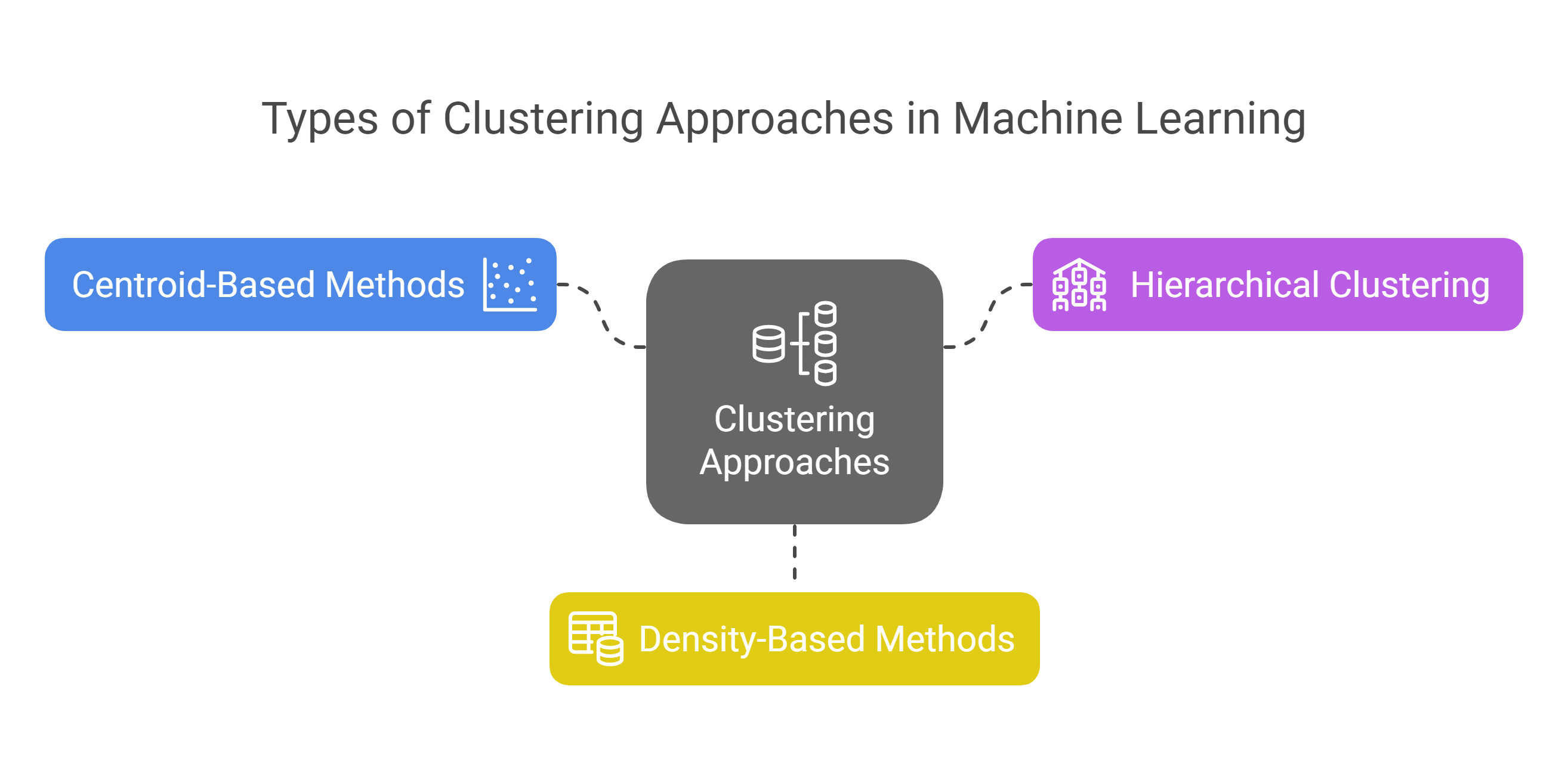
Clustering approaches in machine learning differ based on how they group data. Centroid-based methods like K-Means use centroids to assign data points to clusters, working well for spherical data but struggling with irregular shapes. Hierarchical clustering creates a tree-like structure, merging or splitting clusters, offering flexibility and clear visual insights. 

Density based methods like DBSCAN, OPTICS, and HDBSCAN group data based on areas of high density, making them ideal for complex shapes and noisy data. Here is a quick overview of the types of clustering approaches:

1. Centroid-based: K-Means

K-Means is a popular centroid-based clustering algorithm that divides data into a pre-defined number of clusters. It works by finding each cluster's centroid (mean) and assigning data points to the nearest centroid. It's fast, computationally efficient, and performs well when the data has distinct, spherical-shaped clusters.

Example: Suppose you’re analyzing ride data for a cab service. K-Means could be used to group trips based on location, fare, and distance. For instance, it could create short-distance, medium-distance, and long-distance ride clusters. This helps identify areas where cab demand is highest and optimize fleet allocation.

K-Means is particularly useful for segmentation tasks where the number of clusters is known in advance, and the data naturally falls into well-separated groups.

Why It Helps:

• Efficiency: It’s a quick, straightforward algorithm that works well with large datasets.
• Clear Structure: This is ideal for cases where data points belong to one of the predefined groups, like market segmentation.
• Interpretability: The results are easy to interpret, as each cluster has a clear centroid representing its center.

Where It Lacks: K-Means assumes clusters are spherical and equally sized, which limits its accuracy with real-world data. It struggles with irregular shapes, overlapping regions, or noise. For example, trips in high-traffic areas in ride data may form complex patterns that K-Means can't capture. In such cases, DBSCAN performs better by identifying clusters based on density, not distance from a center.

Also Read: K Means Clustering in R: Step-by-Step Tutorial with Example

2. Hierarchical Clustering

Hierarchical clustering builds a tree-like structure of nested clusters. The two main types are:

• Agglomerative: Starts with individual data points and progressively merges the closest clusters.
• Divisive: It begins with all data points in one cluster and recursively splits into smaller groups.

Example: In the telecom industry, you might use agglomerative clustering to group users based on call duration and data usage. This method helps you visualize user segments in a dendrogram (tree-like structure), making it easier to see relationships between different groups, such as light, medium, and heavy users. This visual approach is handy when understanding how clusters merge or split based on data points.

Why It’s Useful:Hierarchical clustering is valuable for its flexibility and ability to produce a detailed, multi-level view of clusters. It's beneficial in exploratory data analysis, where you want to see a range of possible cluster divisions at different levels of granularity. For example, you can use it to segment users into broad categories, then drill down into more specific sub-groups.

Where It Lacks:However, hierarchical clustering can struggle with large datasets, as its time complexity grows exponentially with the number of data points. It also doesn’t perform well when clusters vary widely in size, shape, or density, making it less suitable for more complex clustering tasks than density-based methods like DBSCAN or HDBSCAN.

Also Read: Understanding the Concept of Hierarchical Clustering in Data Analysis: Functions, Types & Steps

3. Density-based clustering

Density based methods group data based on areas of high point concentration. These techniques don’t assume any particular cluster shape.

Example: Suppose you're analyzing location data for a city’s emergency response team. DBSCAN can detect clusters of incidents in dense areas like traffic-heavy roads and flags outlier events in remote zones, something K-Means would miss.

• DBSCAN efficiently finds clusters of any shape, especially in spatial data.
• OPTICS improves DBSCAN by better handling varying densities.
• HDBSCAN offers hierarchical output and works well even with noisy or uneven data.

Struggling to uncover patterns in unlabelled data? Unlock the power of unsupervised learning with UpGrad’s free course on clustering. Master K-Means, Hierarchical Clustering, and advanced techniques to solve real-world problems and enhance your data analysis skills.

Limitations of Traditional Methods

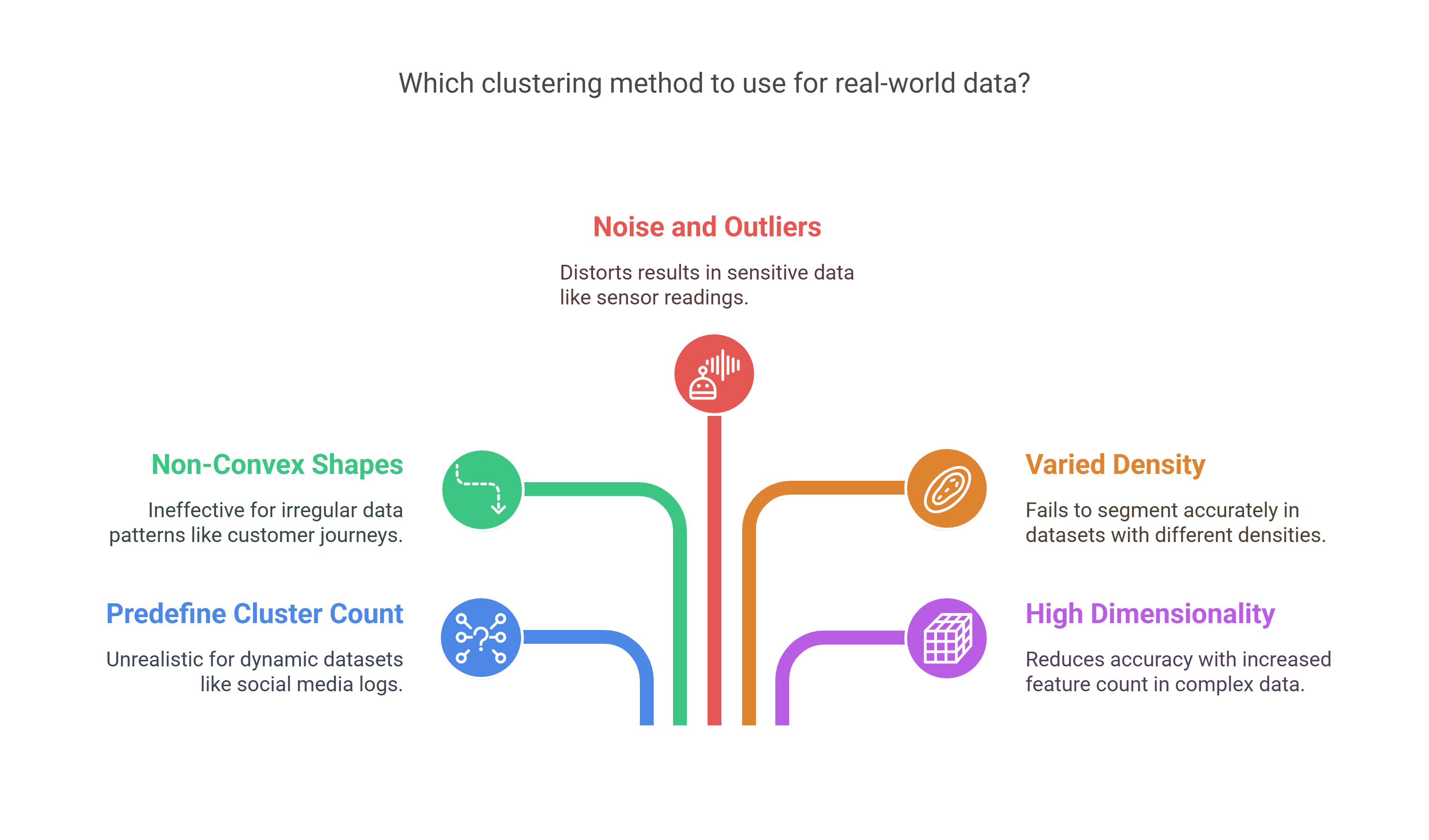
Traditional clustering methods, like K-Means and hierarchical clustering, can struggle with real-world data. They often require you to predefine the number of clusters, fail with non-convex shapes, and are sensitive to noise and outliers. These methods also struggle with varying-density clusters, making them less effective in complex data scenarios. Here are the limitations of traditional approaches:

• Require you to predefine cluster count: In dynamic datasets, like social media behavior logs, it’s unrealistic to assume a fixed number of user groups.
• Fail with non-convex shapes: In customer journey data, user paths might not follow regular patterns, making centroid methods ineffective.
• Sensitive to noise and outliers: If you're clustering sensor data from a smart irrigation system, faulty readings can significantly distort the results.
• Struggle with varied density: For datasets where clusters have different densities, like income levels across urban and rural districts, traditional methods fail to segment accurately.
• High dimensionality worsens accuracy: As feature count increases in genomics or text data, traditional methods become less reliable.

Also Read: How does Unsupervised Machine Learning Work?

Now that you have a solid understanding of clustering and density based methods, let's break down the different density based methods.

Types of Density-Based Methods

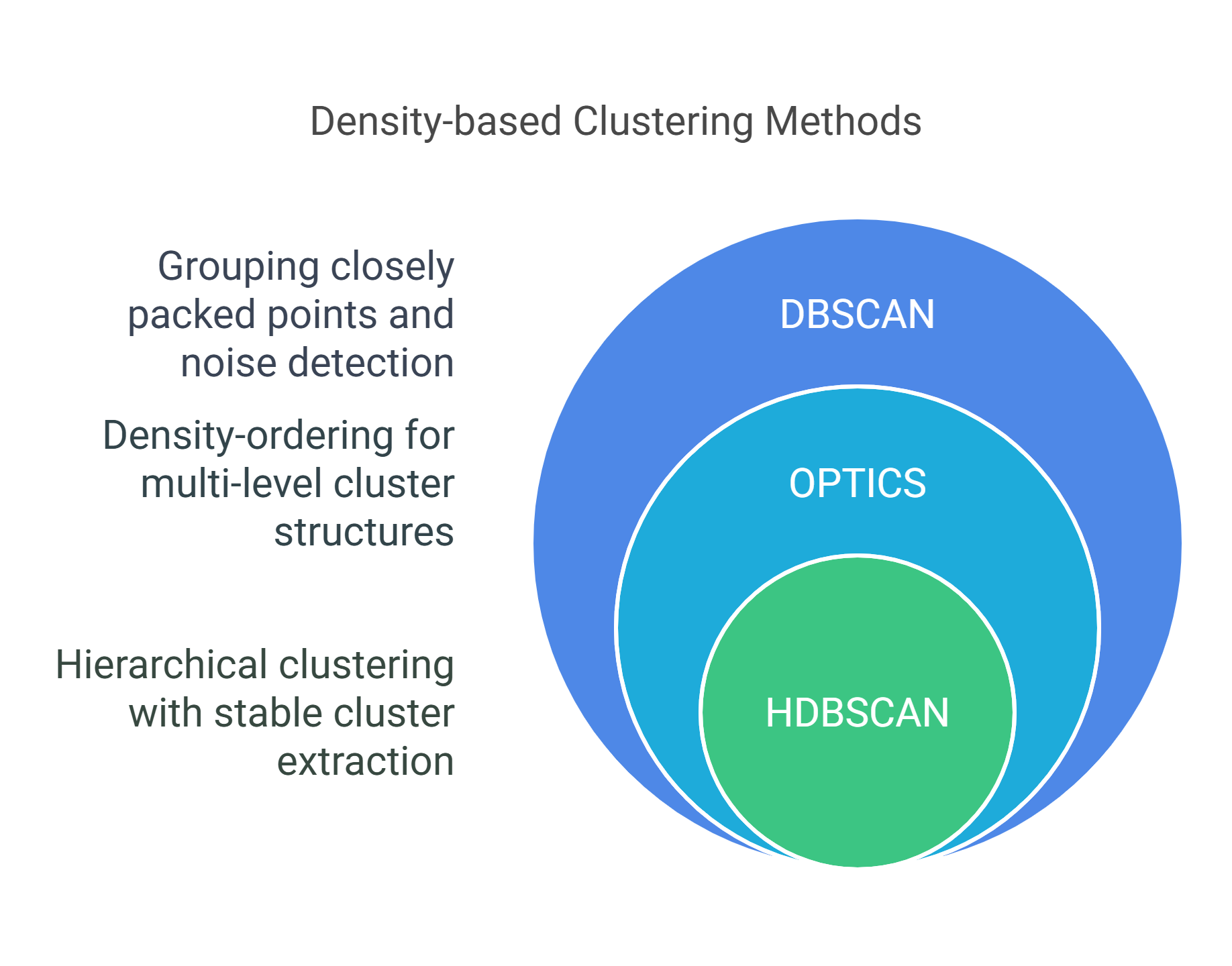
Density based methods differ in defining dense regions and managing cluster shape and noise variations. DBSCAN finds clusters by grouping closely packed points and labeling outliers as noise. OPTICS improves on DBSCAN by ordering points to reveal cluster structures across multiple density levels, making it more flexible. HDBSCAN builds a hierarchy of clusters and extracts the most stable ones, eliminating the need to set a distance threshold manually.

Each method offers a unique way to handle real-world challenges like irregular shapes, noise, and varying densities. Let’s break down three major algorithms that use this approach and explore how they solve real clustering challenges.

1. DBSCAN 

DBSCAN (Density-Based Spatial Clustering of Applications with Noise) is a machine learning clustering algorithm that groups data points based on their density in a dataset. It identifies clusters of varying shapes and sizes by evaluating the number of points within a given radius. However, DBSCAN can struggle with datasets with differing densities, as it assumes that clusters are roughly similar in density, which can lead to challenges when dealing with datasets with significantly different cluster densities.

It requires two parameters:

• Epsilon (ε): Epsilon, or ε, is the maximum distance between two points for them to be considered neighbors. It defines the neighborhood size. A smaller ε may result in many small clusters or even label most points as noise. A larger ε can cause distinct clusters to merge, reducing clustering accuracy. Choosing the right ε is key to solving real machine learning problems effectively.
• min_samples: This defines the minimum number of points required to form a dense region, determining whether a point is a core point. A point with fewer than min_samples neighbors within ε is considered a border point or noise, not because it automatically gets labeled as noise, but because it doesn't meet the criteria to form a dense cluster. This distinction is essential, as min_samples controls the core point formation, not just noise classification.

Step-by-Step Process of DBSCAN

1. Select a point randomly: You begin by choosing a data point that hasn’t been visited. This random selection kicks off the clustering process. For example, imagine you're clustering store locations based on customer footfall. You start with one store location and explore how closely others surround it.
2. Check if it has min_samples neighbors within eps: Next, check how many points lie within a distance of ε (epsilon) from the selected point. These are its neighbors. If the count meets or exceeds min_samples, that point is dense enough to be considered a core point. This threshold helps ensure you're identifying meaningful clusters and not random scatterings.

Example: If you’ve set min_samples = 5 and ε = 0.3, the algorithm looks for at least 5 nearby data points within 0.3 units of distance.

3. If yes, it's a core point. Form a cluster: If the point qualifies as a core point, DBSCAN creates a new cluster around it. All directly connected points (neighbors) are added to this cluster. These represent tightly grouped locations, events, or items, say, high-activity ATM spots in a metro city.
4. Expand the cluster by including density-reachable points: The cluster is then expanded outward. For each neighbor, DBSCAN checks if that point is also a core point. If it is, its neighbors are also included in the cluster. This process continues recursively and spreads the cluster like a ripple in a pond. Even border points (not dense enough themselves but connected to a core) get absorbed.

Think of this like mapping COVID-19 hotspots: once one area is confirmed as a cluster, you look at nearby zones and include them if they show enough activity.

5. If no, label it as noise or a border point: If the selected point doesn’t have enough neighbors within ε, it's labeled as noise or, if it lies close to a core point, as a border point. Noise points are considered outliers; they don’t belong to any cluster. This is useful in fraud detection or anomaly monitoring, where rare events stand out.
6. Repeat until all points are processed: The algorithm selects unvisited points and repeats the process until every point in your dataset is either assigned to a cluster or labeled as noise. No point is skipped or reprocessed.

Pseudocode:

for point in dataset:
    if point is not visited:
        mark as visited
        neighbors = regionQuery(point, eps)
        if len(neighbors) < min_samples:
            mark as noise
        else:
            expandCluster(point, neighbors)

Implementing DBSCAN in Python

Here’s how you can use the Python library sklearn to run DBSCAN. You can also use matplotlib.pyplot to visualize the clusters in your dataset.

1. Import Libraries 

import matplotlib.pyplot as plt
import numpy as np
from sklearn.cluster import DBSCAN
from sklearn import metrics
from sklearn.datasets import make_blobs
from sklearn.preprocessing import StandardScaler
from sklearn import datasets

2. Prepare the Dataset

You'll create a dataset using sklearn to model clustering. Use the make_blobs function to generate sample data with clear cluster structures for testing.

# Load data in X
X, y_true = make_blobs(n_samples=300, centers=4,
                       cluster_std=0.50, random_state=0)

3. Modeling The Data Using DBSCAN 

db = DBSCAN(eps=0.3, min_samples=10).fit(X)
core_samples_mask = np.zeros_like(db.labels_, dtype=bool)
core_samples_mask[db.core_sample_indices_] = True
labels = db.labels_

# Number of clusters in labels, ignoring noise if present.
n_clusters_ = len(set(labels)) - (1 if -1 in labels else 0)

# Plot result

# Black removed and is used for noise instead.
unique_labels = set(labels)
colors = ['y', 'b', 'g', 'r']
print(colors)
for k, col in zip(unique_labels, colors):
    if k == -1:
        # Black used for noise.
        col = 'k'

    class_member_mask = (labels == k)

    xy = X[class_member_mask & core_samples_mask]
    plt.plot(xy[:, 0], xy[:, 1], 'o', markerfacecolor=col,
             markeredgecolor='k',
             markersize=6)

    xy = X[class_member_mask & ~core_samples_mask]
    plt.plot(xy[:, 0], xy[:, 1], 'o', markerfacecolor=col,
             markeredgecolor='k',
             markersize=6)

plt.title('number of clusters: %d' % n_clusters_)
plt.show()

Code Explanation: You apply the DBSCAN clustering algorithm to your dataset X using eps=0.3 and min_samples=10. After fitting the model, you extract the labels assigned to each data point. Points labeled -1 are identified as noise, while others belong to detected clusters. You then create a mask to separate core points from border points based on DBSCAN’s internal classification.

The number of clusters is calculated by counting the unique labels, excluding noise. Finally, you visualize the clusters using matplotlib. Each cluster is shown differently, and noise points are displayed in black. Core points are plotted with one marker style, and border points with another, helping you understand how DBSCAN grouped the data spatially.

Output:

Pros

• Identifies clusters of arbitrary shapes
• Can detect outliers effectively
• Doesn’t need the number of clusters as input

Cons

• Very sensitive to eps and min_samples
• Doesn’t perform well with varying cluster densities

Struggling with data manipulation and visualization? Check out upGrad’s free Learn Python Libraries: NumPy, Matplotlib & Pandas course. Gain the skills to handle complex datasets and create powerful visualizations. Start learning today!

Also Read: What is Cluster Analysis in Data Mining? Methods, Benefits, and More

2. OPTICS 

OPTICS (Ordering Points to Identify the Clustering Structure) is a density-based clustering algorithm that enhances DBSCAN by better handling clusters with varying densities. Unlike DBSCAN, OPTICS doesn’t require specifying the number of clusters beforehand. It orders data points based on their reachability distance, which reveals the clustering structure at multiple density levels. 

This ability to capture clusters of different shapes and densities makes OPTICS more flexible and practical for complex datasets.

Key Concepts

1. Reachability Distance: This is the distance required to reach a point from another, considering the density of points around them. If points are in a dense region, the reachability distance between them will be smaller.
2. Core Distance: Based on its min_samples and eps parameters, the core distance is the minimum distance to make each point a core point. It's critical in determining the density of regions.

Why OPTICS?

OPTICS addresses the sensitivity of DBSCAN to the eps parameter by providing a reachability plot that allows you to observe clusters at various densities. This helps identify clusters even when DBSCAN might fail due to inappropriate eps values. Additionally, since OPTICS does not need you to set eps directly, it can be more robust and reliable across datasets with varying cluster densities.

Step-by-Step Process of OPTICS

1. Select a point randomly: As with DBSCAN, you start by selecting a random data point from the dataset.
2. Calculate reachability distances: For the selected point, OPTICS calculates the reachability distance to other points based on density and the eps parameter.
3. Expand the region: Once a point has its reachability distances calculated, OPTICS continues expanding outward to include other points in the cluster, while considering their core distances.
4. Order the points: Unlike DBSCAN, OPTICS generates an ordered list of points based on reachability distances, showing how points relate to one another in density.
5. Construct the reachability plot: The reachability plot is a visual representation of these distances, and by analyzing it, you can identify clusters and noise at different density levels.

Pseudocode:

for point in dataset:
    if point is not visited:
        mark as visited
        neighbors = regionQuery(point, eps)
        if len(neighbors) < min_samples:
            mark as noise
        else:
            expandCluster(point, neighbors)
            orderPointsByReachability()

Implementing OPTICS in Python

Here’s how you can implement OPTICS using sklearn:

import matplotlib.pyplot as plt
import numpy as np
from sklearn.cluster import OPTICS
from sklearn.datasets import make_blobs

# Prepare the dataset
X, y = make_blobs(n_samples=300, centers=4, cluster_std=0.60, random_state=0)

# Initialize OPTICS
optics = OPTICS(min_samples=10, xi=.05, min_cluster_size=0.1)

# Fit the model
optics.fit(X)

# Plot the result
labels = optics.labels_
unique_labels = set(labels)
colors = ['y', 'b', 'g', 'r']

for k, col in zip(unique_labels, colors):
    if k == -1:
        col = 'k'  # black is used for noise
    
    class_member_mask = (labels == k)
    xy = X[class_member_mask]
    
    plt.plot(xy[:, 0], xy[:, 1], 'o', markerfacecolor=col, markeredgecolor='k', markersize=6)

plt.title('OPTICS Clustering')
plt.show()

Code Explanation:

1. Preparing the dataset: Like DBSCAN, you create a dataset with make_blobs to simulate a real-world clustering problem.
2. Fitting the model: You use OPTICS from sklearn to fit the model to your dataset. min_samples defines the minimum number of points needed to form a dense region, and xi and min_cluster_size help determine the density levels to capture different clusters.
3. Plotting the clusters: The result is visualized similarly to DBSCAN, with different colors representing different clusters and black indicating noise.

Output: 

Pros:

• Can handle varying densities: Unlike DBSCAN, OPTICS doesn’t require setting eps, making it more flexible with datasets with clusters of different densities.
• Provides detailed clustering structure: The reachability plot and ordered points give a better understanding of the dataset's structure.
• Detects outliers effectively: It labels points that don’t fit into any cluster as noise.

Cons:

• Computationally expensive: OPTICS can be slower than DBSCAN, especially for larger datasets.
• Requires careful parameter tuning: While more flexible than DBSCAN, choosing the right min_samples, xi, and min_cluster_size parameters still involves experimentation.

Also Read: Clustering vs Classification: What is Clustering & Classification

3. HDBSCAN 

HDBSCAN is an extension of DBSCAN that combines hierarchical clustering with the core principles of density-based clustering. Unlike DBSCAN, which requires a fixed distance parameter (ε), HDBSCAN creates a hierarchy of clusters by varying the density threshold, allowing it to handle cluster shapes, sizes, and densities more effectively.

The key innovation in HDBSCAN is its stability-based cluster selection. After building a hierarchy, HDBSCAN evaluates how persistent each cluster is across different density levels. This persistence is quantified as a measure of cluster stability that remains intact over a wide range of thresholds, and is considered more stable and meaningful. The algorithm then selects the most stable clusters from the hierarchy, filtering out noise and unstable groupings.

Key Features of HDBSCAN:

• Hierarchical Clustering: HDBSCAN creates a hierarchical tree (dendrogram) of clusters at varying density levels, which can be used to extract clusters at different granularity levels.
• Stability-based Clustering: After building the hierarchy, HDBSCAN examines each cluster's stability (how consistent it is across varying densities) and selects the most stable clusters, eliminating unnecessary noise.
• No Need for eps: Unlike DBSCAN, HDBSCAN doesn't require you to set eps. Instead, it finds the optimal density thresholds independently, making it easier to use for more complex datasets.

Step-by-Step Process of HDBSCAN

1. Building the Cluster Tree: HDBSCAN starts by ordering the points based on their mutual reachability (a measure of how close points are in terms of density). It then constructs a dendrogram to capture the clustering hierarchy at various density levels.
2. Condensing the Tree: Once built, HDBSCAN looks for stable clusters across a wide range of density values. Stability is defined as how consistently the cluster remains as the density threshold changes.
3. Extracting Stable Clusters: The algorithm selects the most stable clusters and eliminates noise points and less stable clusters. This results in clusters well-separated from noise, even in datasets with varying density.
4. Labeling Points: After extracting the stable clusters, each point is assigned to one of the identified clusters or labeled as noise. The noise points are those that do not meet the density threshold at any level.

Pseudocode:

# Step 1: Compute mutual reachability distances between points
distances = compute_mutual_reachability(X)

# Step 2: Construct the hierarchy of clusters (dendrogram)
dendrogram = build_cluster_hierarchy(distances)

# Step 3: Condense the hierarchy by removing less stable clusters
stable_clusters = extract_stable_clusters(dendrogram)

# Step 4: Assign points to clusters based on stability
for point in X:
    if point belongs to a stable cluster:
        assign point to that cluster
    else:
        label point as noise (if no stable cluster)

Plotting HDBSCAN Clusters in Python:

Here's how you can implement HDBSCAN and plot the resulting clusters using Python:

import matplotlib.pyplot as plt
import numpy as np
import hdbscan

# Create a dataset
X, _ = make_blobs(n_samples=300, centers=4, cluster_std=0.60, random_state=42)

# Perform HDBSCAN clustering
clusterer = hdbscan.HDBSCAN(min_cluster_size=10)
labels = clusterer.fit_predict(X)

# Plot results
plt.figure(figsize=(8, 6))
plt.scatter(X[:, 0], X[:, 1], c=labels, cmap='Spectral')
plt.title('HDBSCAN Clustering')
plt.show()

Code Explanation:

• HDBSCAN Setup: You initialize the HDBSCAN model by specifying min_cluster_size=10, which means that the smallest cluster that can be formed will contain at least 10 points.
• Fitting the Model: The model is fitted on the dataset, and the fit_predict method assigns cluster labels to each data point.
• Visualization: Using matplotlib, you plot the data points, coloring them according to their cluster label. Noise points are typically labeled as -1 and appear in a distinct color.

Output:

Pros of HDBSCAN:

• Handles datasets with varying densities better than DBSCAN.
• Automatically determines the optimal density threshold.
• Produces a hierarchical structure that can be useful for multi-level clustering.

Cons of HDBSCAN:

• More computationally expensive than DBSCAN.
• The algorithm’s performance can degrade with very high-dimensional data or large datasets.
• Sensitive to the min_cluster_size parameter, which requires careful tuning.

If you want to build a higher-level understanding of Python, upGrad’s Learn Basic Python Programming course is what you need. You will master fundamentals with real-world applications & hands-on exercises. Ideal for beginners, this Python course also offers a certification upon completion.

Now that you have a clear understanding of the different types of density based methods, let's look at the practical applications of density based clustering.

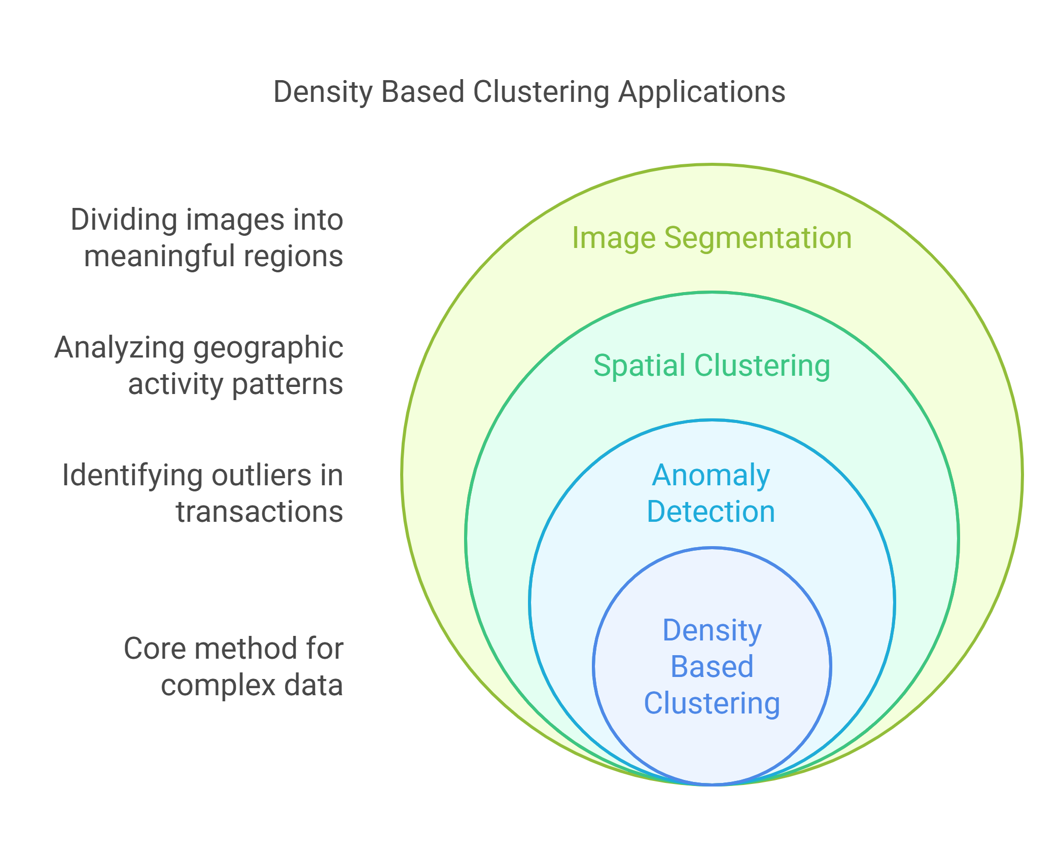
Practical Applications of Density-Based Clustering

In real-world datasets, you often encounter noise, irregularities, and complex structures that traditional clustering methods fail to handle. Density based clustering gives you the flexibility to work with such complexity without guessing how many clusters to expect.

Here’s how you can apply these methods in high-impact areas, with real examples from Indian industries and public services:

1. Anomaly Detection

You can use density based clustering to identify fraud in financial transactions by detecting behavioral outliers such as sudden high-value transfers, unusual login times, rapid spending spikes, transactions from unknown devices, or access from unexpected geographic locations.

When you apply DBSCAN, it treats densely packed, repetitive behavior as usual. Unusual actions like sudden high-value transfers from unfamiliar devices or abnormal geolocation don’t belong to any dense group. These become noise points, which you can review as potential fraud.

Example: A Bengaluru FinTech firm used DBSCAN to cluster UPI transactions based on time, amount, and location. DBSCAN’s ability to identify dense clusters and isolate sparse, unusual points made it ideal for detecting anomalies in financial behavior. It flagged outliers like unexpected transfers at odd hours or from unfamiliar locations as potential fraud. This approach reduced false positives by focusing on behavioral patterns rather than rigid rules, avoiding false alarms from one-time large payments by trusted users.

2. Spatial Clustering

You can use density based clustering to analyze spatial data by identifying regions where activities are geographically concentrated. This helps you detect meaningful location patterns such as high-traffic zones, service hotspots, or under-served areas, without setting predefined boundaries.

Applying DBSCAN to latitude and longitude data forms clusters based on how close and dense the data points are. Areas with frequent activity, like delivery drop-offs or vehicle stops, form dense clusters. Isolated points, such as rare stops in low-traffic zones, are treated as noise or exceptions.

Example: Esri India used DBSCAN on spatial data to analyze event locations across Western and Southern India. By setting a minimum of 100 events per cluster and a 20-kilometer search radius, they found 15 dense clusters in regions like Coastal Maharashtra, Goa, and Kerala. This method revealed that 80% of events in the five years were concentrated in these clusters, guiding resource deployment and service planning.

3. Image segmentation

Density-based clustering, like DBSCAN, is ideal for image segmentation, especially when irregular boundaries or objects overlap. Unlike traditional methods, DBSCAN groups pixels based on proximity and feature similarity, such as color, intensity, or texture.

1. Feature Selection: Important image features like pixel intensity, color, and texture are extracted for clustering. These help distinguish between objects and the background.
2. Clustering Process: DBSCAN identifies "core" pixels with enough neighbors within a set radius. These core pixels form clusters, grouping similar pixels based on density, allowing for the segmentation of meaningful structures.
3. Handling Outliers: DBSCAN identifies pixels with too few neighbors as outliers, such as noise or edges, and excludes them from clusters, making it robust in noisy images.
4. Adapting to Irregular Boundaries: Unlike methods like k-means, DBSCAN doesn’t assume specific shapes. It can segment complex regions with poorly defined boundaries.

Example: In 2024, a team applied a modified HDBSCAN algorithm to segment hyperspectral images of cotton crops. It grouped pixel data into dense clusters representing healthy and stressed areas. This helped you detect early signs of disease more accurately. The approach improved early disease detection rates by 18 percent compared to rule-based segmentation, giving farmers better tools for timely crop monitoring.

Also Read: Image Segmentation Techniques [Step By Step Implementation]

4. Genomics & NLP

You can use density based clustering to uncover hidden patterns in genomic sequences or natural language data by working with high-dimensional embeddings. Genomics often encodes gene expression profiles or mutation patterns into dense vectors. Similarly, sentence or document embeddings from models like BERT capture deep semantic relationships in NLP.

When you apply methods like DBSCAN, they can group biologically or semantically similar data points without needing predefined categories. Dense regions in the embedding space represent common structures or themes, while sparse regions often capture rare mutations or outlier topics.

Example: In 2025, a news aggregator in Bengaluru applied BERTopic with HDBSCAN to Kannada news articles. This approach grouped articles into clear themes, even when topics overlapped or appeared infrequently. Compared to their earlier LDA-based system, you would see a 40% boost in topic coherence and quicker detection of emerging local issues.

Struggling to make sense of how machines understand language? Dive into UpGrad's free Natural Language Processing courses! Learn tokenization, spell correction, phonetic hashing, and more to create AI-driven applications.

Also Read: Anomaly Detection and Outlier Detection: Techniques, Tools & Use Cases

Now that you’ve seen how density based clustering works in real-world scenarios, it’s essential to understand the key benefits and challenges you’ll face when using it in machine learning.

Benefits and Challenges of Density Based Clustering in ML that You Must Kno

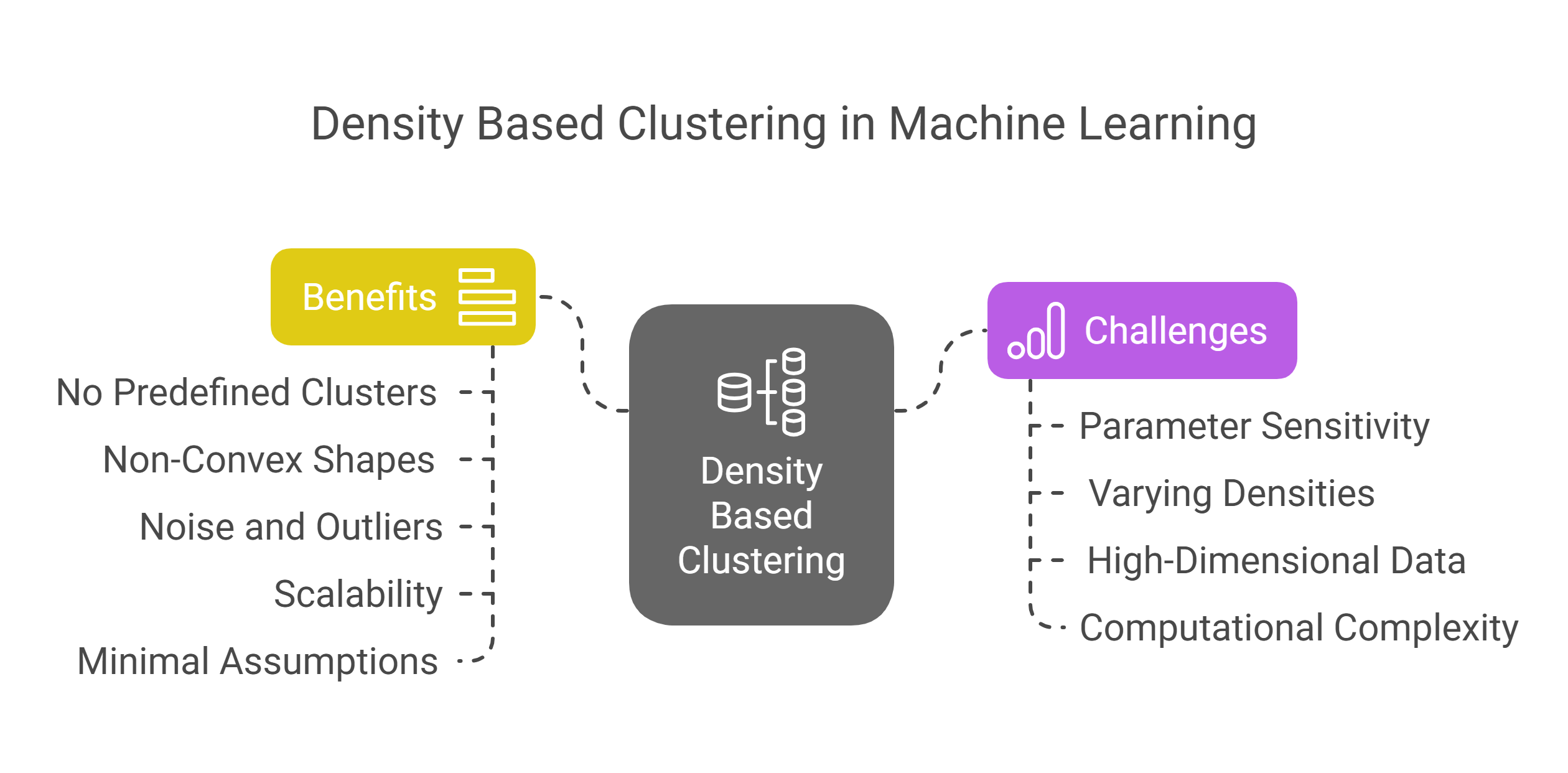
Density based clustering gives you a flexible way to group data based on structure, not assumptions. Unlike traditional methods like k-means, you don’t need to guess the number of clusters or assume circular shapes. This makes it well-suited for messy, real-world datasets, whether you're working with GPS coordinates, financial behavior, or textual embeddings.

To use these methods effectively, you should understand what they do best and where they can create difficulties in applied machine learning scenarios.

Benefits of Density Based Clustering in Machine Learning

• No need to predefine the number of clusters: Unlike k-means or hierarchical clustering, density based methods like DBSCAN and HDBSCAN automatically identify the number of clusters your data contains. This is useful when dealing with dynamic or unlabeled datasets.
• Works well with non-convex shapes: You can handle irregularly shaped clusters, like rings, spirals, or U-shaped patterns, that break traditional algorithms. This is particularly useful in geospatial clustering or genomic data analysis.
• Effective with noise and outliers: Density based clustering naturally separates noisy points or outliers without needing extra preprocessing. This helps with financial fraud data or network intrusion logs, where anomalies are important.
• Scales to large and high-dimensional data: With optimized implementations and dimensionality reduction techniques, density based methods can be applied to real-world datasets like image embeddings or IoT sensor logs.
• Minimal assumptions about data distribution: You don’t need to assume that your data follows a Gaussian distribution or that clusters are equally sized. This makes these methods more flexible in practical deployments.

Challenges of Density Based Clustering in Machine Learning

• Parameter sensitivity: You need to carefully tune parameters like eps, neighborhood radius, and minPts. Poor choices can lead to missed clusters or meaningless groupings. This tuning becomes tricky in multi-modal datasets.
• Difficult to use with varying densities: If your dataset contains clusters of different densities, DBSCAN might fail to separate them. HDBSCAN can handle this better, but still requires validation with real data.
• Not ideal for very high-dimensional data without preprocessing: Distance measures used in density based clustering lose meaning as dimensions grow. You often need to reduce dimensions first, such as with PCA or t-SNE, to get good results.
• Computational complexity in large-scale use: Although efficient for moderate sizes, DBSCAN’s worst-case performance can be expensive on massive datasets without indexing, such as in retail clickstream analysis or telco usage logs.
• Requires spatially meaningful features: Density based methods rely on distance, so your input features must reflect real-world closeness. In text or categorical data, embeddings are often required before clustering can work.

Also Read: What Are IOT Devices?: Definition, Uses, Types

How Can upGrad Help You Become an Expert in Machine Learning?

To effectively apply density based methods like DBSCAN, OPTICS, and HDBSCAN, you need a solid grasp of unsupervised learning, clustering logic, and data preparation. These methods work best when you deal with noisy, unstructured, or irregularly shaped data, especially in real-world domains like finance, geospatial analysis, genomics, and NLP.

Trusted by data professionals, upGrad offers courses that guide you through using Density based methods for practical tasks like anomaly detection and pattern recognition, helping you build effective clustering models for complex data.

In addition to the courses mentioned, here are some more resources to help you further elevate your skills: 

• Artificial Intelligence in the Real World
• Learn Basic Python Programming
• Fundamentals of Deep Learning and Neural Networks

Not sure where to go next in your ML journey? upGrad’s personalized career guidance can help you explore the right learning path based on your goals. You can also visit your nearest upGrad center and start hands-on training today!  

FAQs

1. What challenges arise when applying density based clustering to high-dimensional data?

In high-dimensional spaces, density becomes less meaningful, making it harder for algorithms like DBSCAN to distinguish clusters from noise. This issue, known as the "curse of dimensionality," can lead to poor clustering results. Techniques like PCA (Principal Component Analysis) are often used to reduce dimensions and improve clustering performance.

2. How does DBSCAN handle overlapping clusters and varying densities?

DBSCAN can struggle with overlapping clusters and varying densities, as it may merge nearby clusters or fail to distinguish subtle ones. Tuning parameters like epsilon and MinPts can help, but in cases with significant overlap or density variation, methods like HDBSCAN or combining DBSCAN with techniques like Gaussian Mixture Models (GMM) are often more effective for better separation of clusters.

3. How does HDBSCAN handle noisy data compared to DBSCAN?

HDBSCAN improves on DBSCAN's ability to handle noisy data by employing hierarchical clustering, which can identify clusters at multiple density levels. While DBSCAN may classify many points as noise in a noisy dataset, HDBSCAN can identify smaller clusters that DBSCAN would miss. By considering global and local density variations, HDBSCAN allows you to detect clusters even in noisy datasets where DBSCAN might struggle.

4. How does OPTICS improve clustering over DBSCAN for datasets with varying densities?

OPTICS addresses the problem of varying densities, which DBSCAN struggles with. While DBSCAN uses a fixed epsilon radius, OPTICS does not require this. Instead, OPTICS computes a reachability distance for each point and uses it to generate a hierarchical ordering of points. This allows it to discover clusters of varying densities and to separate dense regions that DBSCAN might merge. As a developer, you can visualize the reachability plot to understand the cluster structure better, making OPTICS more versatile for complex datasets.

5. Can density-based clustering methods be used for high-dimensional data?

Density-based clustering methods like DBSCAN can struggle with high-dimensional data due to the curse of dimensionality, where distance measures become less meaningful in high-dimensional spaces. However, you can improve performance by using dimensionality reduction techniques, such as PCA (Principal Component Analysis) or t-SNE, before applying DBSCAN or OPTICS. 

6. What is the role of the distance metric in density-based clustering?

The distance metric is crucial in determining the success of density-based clustering methods. DBSCAN, OPTICS, and HDBSCAN rely on distance measures (typically Euclidean) to define proximity between points. However, you can adapt these methods with alternative distance metrics, such as cosine similarity for text data or Jaccard distance for binary/categorical data. 

7. Is there any performance difference between DBSCAN and HDBSCAN for large datasets?

DBSCAN is generally faster and more memory-efficient for large datasets, as it only requires a simple density calculation. However, its performance can degrade with datasets that have varying densities. HDBSCAN, while more accurate for complex datasets, is more computationally expensive due to its hierarchical nature. As a developer, you may prefer DBSCAN for speed when dealing with large, uniform datasets. Still, if your data has varying densities, HDBSCAN might provide better results, albeit with slightly higher computational costs.

8. Can OPTICS be used to cluster streaming data?

OPTICS is not inherently designed for streaming data but requires a batch processing approach. However, using incremental clustering or sliding window methods, you can adapt OPTICS to work with streaming data. This involves maintaining a dynamic cluster set that updates as new data points arrive. For real-time applications like fraud detection or sensor data analysis, you can combine OPTICS with online clustering approaches to achieve near-real-time performance.

9. How do I handle density-based clustering for imbalanced datasets?

Density-based clustering methods, especially DBSCAN, can have difficulty with imbalanced datasets because they may classify many points from smaller clusters as noise. To improve performance on imbalanced data, you can adjust the MinPts parameter to account for varying densities. Alternatively, using weighted DBSCAN or combining DBSCAN with other clustering algorithms like K-Means can help better detect smaller or imbalanced clusters. 

10. How can I visualize density-based clustering results effectively?

Visualizing density-based clustering results can be challenging, especially for high-dimensional data. You can reduce dimensionality with PCA or t-SNE and use scatter plots for 2D/3D data. For OPTICS or HDBSCAN, reachability plots or hierarchical trees help understand cluster relationships. Tools like matplotlib, seaborn, and Plotly are great for visualizing in Python.

11. How does DBSCAN differ from K-Means clustering?

Unlike K-Means, DBSCAN can detect clusters of arbitrary shapes and doesn't require the number of clusters to be specified in advance. It can also identify outliers as noise rather than forcing them into clusters. DBSCAN adapts to varying densities, making it more flexible than K-Means, which assumes spherical clusters. However, DBSCAN can be sensitive to parameter choices like epsilon and MinPts, and may struggle with clusters of varying densities or excessive noise.