Probabilistic Clustering in Machine Learning: Exploring Model-Based Approaches

Did you know that Possibilistic Clustering for Probability Density Functions (PCF), introduced in 2024, achieved up to 100% accuracy on simulated data and high G-mean scores on image datasets?

This means PCF is highly effective in detecting patterns and handling outliers, making it more robust than traditional clustering algorithms.

Probabilistic Clustering in Machine Learning refers to algorithms that assign data points to clusters based on probability distributions. Unlike traditional methods, model-based approaches assume underlying data models to describe the clusters.

How does this impact practical applications, such as anomaly detection or image segmentation? By using probabilistic models, this technique provides more flexibility and robustness, especially in complex, real data.

In this blog, we’ll explore various model-based approaches and their significance in probabilistic clustering, highlighting key algorithms and their applications in machine learning.

Elevate your career with upGrad’s Artificial Intelligence & Machine Learning - AI ML Courses, designed in collaboration with the world’s top 1% universities. Join over 1,000 leading companies and unlock an average 51% salary hike while learning from industry experts.

What is Probabilistic Clustering in Machine Learning?

Probabilistic Clustering in Machine Learning, also known as distribution-based clustering, assigns data points to clusters based on probability distributions. In this approach, each data point has a probability of belonging to multiple clusters, instead of being strictly assigned to one. This allows for flexibility in handling uncertainty and overlap between clusters.

Probabilistic clustering models, like Gaussian Mixture Models (GMM) or Expectation-Maximization (EM), assume that the data is generated from a mixture of underlying probability distributions. The model evaluates the likelihood of each point belonging to these distributions and assigns a soft membership based on that probability.

Looking for next leap in your career? upGrad offers several programs that delve into clustering techniques within machine learning, providing both foundational and advanced knowledge.

• Executive Diploma in Machine Learning and AI with IIIT-B
• Master’s Degree in Artificial Intelligence and Data Science

Importance of Probabilistic Clustering in Machine Learning

Probabilistic clustering in machine learning provides a more flexible approach. Unlike other methods, it assigns a probability to each data point for multiple clusters. This is helpful when data points overlap or there is uncertainty in cluster membership.

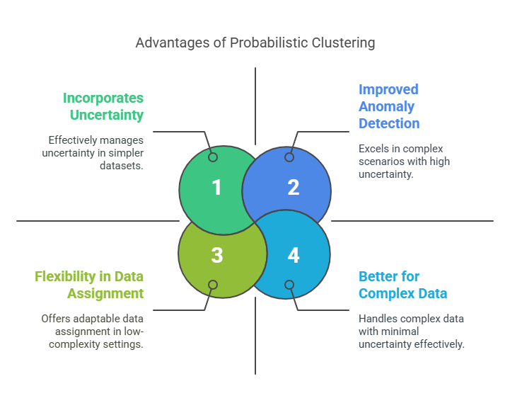
• Flexibility in Data Assignment: Probabilistic clustering in machine learning assigns data points to multiple clusters with varying probabilities, providing a soft classification. This allows for a more nuanced approach, especially when data points exhibit characteristics that span across multiple categories, unlike traditional hard clustering that forces a strict assignment to only one group.
• Handling Overlap: In real-world data, clusters often overlap, making it difficult to assign points to a single group. Probabilistic clustering handles these situations by modeling data points as mixtures of distributions, where each point is allowed to belong to more than one cluster with different likelihoods, ensuring that points lying on the boundaries of clusters are treated more effectively.
• Better for Complex Data: Probabilistic clustering is well-suited for complex datasets where clear boundaries between clusters do not exist. By modeling the data as a distribution, it accommodates intricate patterns and relationships that are difficult for traditional methods to capture, such as overlapping or non-linearly separable data.
• Improved Anomaly Detection: Probabilistic models are particularly effective at identifying outliers, or anomalies, in data. Since each data point has a probability distribution over possible clusters, those with a low likelihood of belonging to any cluster are flagged as anomalies. This method improves detection by focusing on how well points fit into the overall probabilistic model, rather than just their distance from the nearest centroid.
• Incorporates Uncertainty: Probabilistic clustering allows for a more accurate representation of uncertainty within the data. Instead of assigning each point to a single cluster, it quantifies how likely a point is to belong to each cluster, providing a more robust model that accounts for noisy or ambiguous data, thus improving the reliability of the clustering results.

Take your career to the next level with upGrad's Masters in Artificial Intelligence and Machine Learning - IIITB Program. Learn from top faculty and industry experts, and gain hands-on experience with real-world projects and case studies.

Also Read: What is Clustering in Machine Learning and Different Types of Clustering Methods

Having defined probabilistic clustering in machine learning, let’s now examine why distribution-based clustering is crucial for handling the complexities and uncertainties in machine learning tasks.

Why Do We Need Distribution Based Clustering in Machine Learning?

Distribution-based clustering is essential because data often doesn’t fit neatly into predefined clusters. Distribution-based techniques, such as probabilistic clustering, model data as mixtures of probability distributions, providing flexibility.

This allows the algorithm to capture nuanced relationships and handle uncertainties, making it more effective for complex datasets.

Practical Applications Distribution Based Clustering

Distribution-based clustering is widely used in areas where data is complex, uncertain, or overlaps. These methods are particularly effective in customer segmentation, image analysis, and anomaly detection scenarios, where traditional clustering techniques may struggle. Below are several domains where distribution-based clustering provides significant value.

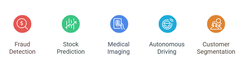
1. Fraud Detection

Probabilistic clustering identifies anomalous patterns in transactional data, flagging potential fraud. By modeling normal transactions as probability distributions, it detects outliers and unusual behavior. For instance, an unusually large international purchase can be flagged as potential fraud if its probability deviates from typical spending patterns.

2. Finance & Stock Prediction

Probabilistic clustering models financial data using probability distributions, capturing complex relationships. It helps in predicting market behavior, identifying investment opportunities, and assessing risk. By analyzing historical stock data, these models detect recurring patterns like price fluctuations, improving forecasting accuracy.

3. Medical Imaging & Healthcare

In healthcare, probabilistic clustering helps segment medical images and identify subtle patterns for disease detection. It enhances image analysis by modeling pixel intensity and assists in early detection of conditions like cancer or heart disease. For example, in MRI scans, it helps differentiate between healthy and abnormal tissues.

4. Autonomous Driving

Probabilistic clustering processes sensor data to detect objects such as pedestrians and vehicles, crucial for real-time decision-making in autonomous driving. It enhances object detection and path planning by modeling environmental data and predicting potential obstacles. This enables vehicles to make adaptive driving decisions based on real-time conditions.

5. Customer Segmentation

In marketing, probabilistic clustering identifies customer groups based on behavior, preferences, and demographics. It enables more personalized marketing by modeling customer data with probability distributions. This approach optimizes product recommendations and helps businesses target segments more effectively, such as offering promotions tailored to high-value customers.

Also Read: Machine Learning Algorithms Used in Self-Driving Cars: How AI Powers Autonomous Vehicles

All of the above applications rely on data mining techniques to extract meaningful insights from complex datasets. Let’s explore how probabilistic model based clustering enhances data mining by providing more accurate, flexible, and reliable results.

Unlock the power of distribution-based clustering and more with the #1 Machine Learning Diploma. Gain expertise in machine learning, Generative AI, and statistics. Enroll today and elevate your career in ML!

Also Read: What is Cluster Analysis in Data Mining? Methods, Benefits, and More

Importance of Probabilistic Model Based Clustering in Data Mining

Probabilistic model based clustering in data mining enables more precise analysis of complex datasets. it allows for data points to belong to multiple clusters simultaneously, providing a more realistic representation of actual data. Probabilistic clustering approach addresses challenges, such as uncertainty, noise, and overlapping data.

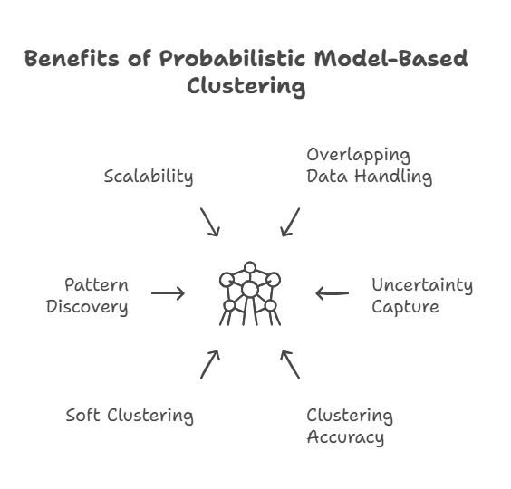
This is how probabilistic clustering helps in data mining:

• Handles Overlapping Data: It effectively manages overlapping clusters, where traditional methods might fail, by allowing data points to belong to more than one cluster with different probabilities.
• Captures Uncertainty in Data: Probabilistic clustering accounts for uncertainty by assigning probabilities to data points, which helps in dealing with ambiguous or noisy data.
• Improves Clustering Accuracy: By modeling data as mixtures of distributions, it improves the accuracy of clustering, particularly for datasets with complex relationships and patterns.
• Enables Soft Clustering: Probabilistic clustering provides soft clustering, where data points have partial membership in multiple clusters, making it ideal for situations where data points do not belong exclusively to one group.
• Enhances Pattern Discovery: It uncovers hidden patterns in data by modeling the underlying distribution, which improves the quality of insights gained through data mining.
• Scalable for Large Datasets: These models can handle high-dimensional and large-scale datasets, making them suitable for modern data mining tasks that involve big data.

Future-proof your tech career with AI-Driven Full-Stack Development. Build AI-powered software using cutting-edge tools like OpenAI, GitHub Copilot, and Bolt AI. Earn triple certification from Microsoft & upGrad, NSDC, and an industry partner, while mastering Leetcode-style problem-solving with 150+ coding challenges. Start today and shape the future of technology!

Also Read: Clustering vs Classification: Difference Between Clustering & Classification

Now that we’ve seen the practical applications of distribution-based clustering, let's explore the models that underpin these techniques and make them effective in machine learning.

Models in Distribution-Based Clustering Methods

In distribution-based clustering, models serve as mathematical representations or assumptions about how data is generated. These models define each cluster as a probability distribution, describing the likelihood of data points belonging to it. They represent clusters as mixtures of distributions, with parameters like means, variances, and mixing coefficients.

Let’s look at the popular models in probabilistic clustering:

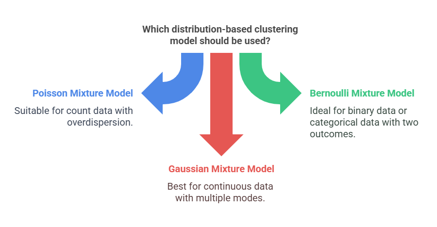
1. Poisson Mixture Mode

The Poisson Mixture Model (PMM) is a probabilistic, distribution-based clustering technique designed for count data, where each data point represents the number of occurrences or events. Instead of assuming all data comes from a single Poisson distribution, the PMM assumes that the data is generated from a mixture of multiple Poisson distributions.

Key Points

• Cluster Representation: The model assumes that each observation is generated from one of several Poisson distributions, with each distribution representing a separate cluster.
• Poisson Parameters: Each cluster is characterized by its own Poisson parameter (λ), representing the mean rate of occurrence.
• Estimation Process: The model estimates mixing proportions (the probability of each cluster) and Poisson parameters (λ values) for each cluster.
• EM Algorithm: The Expectation-Maximization (EM) algorithm is typically used to fit the model, iteratively estimating cluster memberships and parameters until convergence.
• Soft Clustering: Unlike hard clustering, PMM provides probabilities for each observation’s membership in each cluster, enabling soft assignments and handling of overlapping clusters.

Poisson Mixture Model Formula

The Poisson Mixture Model assumes that each data point xi (representing a count) is drawn from one of several Poisson distributions. The model can be expressed mathematically as a mixture of Poisson distributions, where the probability density function (PDF) for a data point xi​ is given by:

P (xi) =k=1k πk​⋅Poisson(xi​∣ λk​)

• Where πk is the mixing proportion for the k^th component (the probability of data coming from the k-th Poisson distribution), with k=1k πk =1
• Poisson (xi​∣ λk​) is the probability mass function (PMF) of the Poisson distribution with parameter λk representing the mean rate of occurrence for the k-th cluster.
• λk is the Poisson parameter (mean) for the k-th component, representing the rate of occurrence of events in that cluster.
• K is the number of clusters.

The Poisson distribution for each cluster is given by: Poisson (xi​∣ λk​)=λkxi e-λk​​xi !

Applications:

• Count Data: Particularly useful for clustering data with overdispersion or zero inflation, such as microbiome data, event logs, or document word counts.
• Healthcare: Applied in predicting health conditions like heart disease by analyzing count-based medical data.
• Biology: Used in modeling genetic or ecological data where counts of species or events are critical.
• Text Mining: Utilized in document classification by clustering word counts or term frequencies.

Also Read: Cluster Analysis in Business Analytics: Everything to know

2. Bernoulli Mixture Model

The Bernoulli Mixture Model (BMM) is a probabilistic clustering technique designed for binary data, where each feature can take a value of either 0 or 1. The BMM assumes that the data is generated from a mixture of multiple Bernoulli distributions. Each corresponding to a different cluster with its own probability profile for each feature. This allows the model to effectively capture the diversity of binary data patterns.

Key Points

• Cluster Representation: Each cluster is modeled as a multivariate Bernoulli distribution, where features are assumed to be independent within each cluster.
• Parameter Estimation: The model estimates the mixing weights, which represent the probability of each data point belonging to each cluster. It also estimates the success probability for each feature within every cluster. This probability is often referred to as the frequency matrix.
• Soft Clustering: The BMM provides soft cluster assignments, meaning each data point has a probability of belonging to each cluster, rather than a hard assignment.
• EM Algorithm: The Expectation-Maximization (EM) algorithm is used to estimate the parameters, iteratively assigning data points to clusters and refining the parameters until convergence.

Bernoulli Mixture Model Formula

The probability of a binary vector X under the BMM is given by the mixture of Bernoulli distributions:

P(X) =k=1k wk l=1L Pklxl ( 1-pkl )1-Xl

• K is the number of clusters,
• wk is the mixing weight for cluster k
• pkl is the probability of feature l being 1 in cluster k,
• L is the number of features,
• xl ​ represents the value of feature l in the binary vector X

Applications

• Survey Responses: Useful for clustering binary survey responses (e.g., yes/no answers).
• Genetic Markers: Applied to clustering the presence/absence of genetic markers in population genetics.
• Document Term Matrices: Effective in document clustering, especially when representing word presence/absence in text mining.
• Image Segmentation: Used for segmenting binary images, such as distinguishing between foreground and background.

3. Gaussian Mixture Model (GMM)

A Gaussian Mixture Model (GMM) is a probabilistic, soft clustering method that assumes data points are generated from a mixture of several Gaussian (normal) distributions. Each distribution represents a cluster, and instead of assigning each data point to a single cluster, GMM estimates the probability that each data point belongs to each cluster. This makes GMM highly effective for datasets with complex, overlapping clusters.

Key Features

• Cluster Representation: Each cluster is modeled as a Gaussian distribution, characterized by a mean (center), covariance (shape/size), and mixing probability (weight).
• EM Algorithm: The model is fitted using the Expectation-Maximization (EM) algorithm, which iteratively estimates the parameters of the Gaussian distributions (mean, covariance) and the membership probabilities of data points.
• Soft Clustering: GMM provides soft clustering, meaning that each data point has a probability of belonging to each cluster. This is unlike hard clustering methods like K-means, which assign each point to exactly one cluster.
• Model Flexibility: GMM can model clusters with different shapes, sizes, and orientations, whereas methods like K-means assume spherical clusters with the same variance.
• Model Selection: The number of components (clusters) in a GMM is typically determined using model selection criteria. Common methods include the Bayesian Information Criterion (BIC) and the Akaike Information Criterion (AIC). These criteria help balance model complexity with data fit, ensuring the model is neither too simple nor too complex.

Gaussian Mixture Model Formula

The probability density function of a Gaussian Mixture Model is given by:

P(x) =k=1k wk ⋅N (x∣μk , k )

Where:

• p(x) is the probability density function for the data point x
• k is the number of clusters (components),,
• k is the number of clusters (components),
• wk is the mixing weight for cluster k,
• N(x∣μk , k) is the Gaussian distribution for cluster k, with mean μk ​ and covariance matrix k

Applications

• Customer Segmentation: GMM segments customers based on behaviors or demographics, enabling targeted marketing.
• Anomaly Detection: GMM identifies outliers, useful in fraud detection or spotting unusual patterns in data.
• Image Segmentation: GMM is used for segmenting images, improving object recognition and classification.
• Speech Recognition: GMMs model speech signals to enhance voice detection and classification.
• Density Estimation: GMM estimates probability densities, aiding in finance and healthcare for modeling data distributions.

Models are mathematical representations or assumptions about how data is generated. Whereas algorithm is the procedure to fit a model to the data. Here are some common algorithms used in probabilistic clustering.

Elevate your career with upGrad's Professional Certificate Program in Business Analytics & Consulting, developed in collaboration with PwC Academy. Gain advanced skills, hands-on experience, and certifications to excel in high-impact analytics and consulting roles.

Algorithms in Probabilistic Clustering in Machine Learning

Probabilistic clustering in machine learning uses statistical methods to group data by modeling each cluster as a probability distribution. Algorithms are the procedures or steps used to fit the model to the data. They estimate the model parameters and assign data points to clusters based on probabilities. Here are some commonly used algorithms:

Expectation-Maximization (EM) Algorithm

The Expectation-Maximization (EM) algorithm is a powerful method used to estimate the parameters of probabilistic models in cases where the data is incomplete, missing, or contains hidden variables. EM works iteratively, improving the model's parameter estimates by alternating between two key steps: Expectation (E-step) and Maximization (M-step).

Key Steps in the EM Algorithm:

1. E-step (Expectation): In this step, the algorithm estimates the "missing" or hidden data based on the current estimates of the model parameters. This is done by calculating the probability (or "responsibility") that each data point belongs to each cluster or component. Essentially, the algorithm evaluates the likelihood of the observed data given the current parameters.
2. M-step (Maximization): Once the hidden data is estimated, the algorithm then maximizes the likelihood by updating the model parameters (such as means, variances, or mixing coefficients). The goal is to find the set of parameters that best explains the observed data.

These two steps are repeated iteratively until the model parameters converge to a stable solution.

Practical Example of EM Algorithm in Gaussian Mixture Model (GMM) clustering

Let's consider a practical example of Gaussian Mixture Model (GMM) clustering, which is commonly fitted using the EM algorithm. Suppose you have a dataset of test scores from students, and you suspect there are two different groups: one group of students with high scores and another with low scores. However, you don’t know which student belongs to which group. You want to use EM to model this situation.

1. Initial Guess: You start by assuming some initial parameters, such as the means and variances of the two groups (clusters).
2. E-step: In this step, the algorithm estimates the probability of each student belonging to the high-score group and the low-score group based on the current parameters.
3. M-step: Next, the algorithm updates the mean and variance of each group based on the probabilities calculated in the E-step. For example, it might adjust the mean of the high-score group to be more accurate based on the students who have a high probability of belonging to that group.
4. Repeat: The E-step and M-step are repeated, and with each iteration, the model improves its estimates of the group memberships and the parameters of each group. Eventually, the algorithm converges to a set of parameters where the likelihood of the data is maximized.

Example Code for GMM Clustering Using the EM Algorithm

import numpy as np
import matplotlib.pyplot as plt
from sklearn.mixture import GaussianMixture

# Step 1: Generate synthetic data (e.g., test scores from two groups: high scores and low scores)
# Group 1: Low scores
low_scores = np.random.normal(loc=60, scale=5, size=(150, 1))  # mean=60, std=5
# Group 2: High scores
high_scores = np.random.normal(loc=85, scale=5, size=(150, 1))  # mean=85, std=5

# Combine both groups to form the complete dataset
X = np.vstack([low_scores, high_scores])

# Step 2: Visualize the data
plt.scatter(X, np.zeros_like(X), s=10, color='blue')  # Scatter plot of the test scores
plt.title("Generated Test Scores")
plt.xlabel("Test Scores")
plt.show()

# Step 3: Fit a Gaussian Mixture Model (GMM) using the EM algorithm
# Assume we know there are 2 clusters (low and high scores)
gmm = GaussianMixture(n_components=2, covariance_type='full', random_state=42)
gmm.fit(X)

# Step 4: Predict cluster membership
labels = gmm.predict(X)

# Step 5: Visualize the GMM clustering results
plt.scatter(X, np.zeros_like(X), c=labels, s=10, cmap='viridis')  # Colored by cluster labels
plt.title("GMM Clustering Results: Low and High Scores")
plt.xlabel("Test Scores")
plt.show()

# Step 6: Check the parameters (means and variances) learned by the model
print("Cluster Means: \n", gmm.means_)
print("Covariances: \n", gmm.covariances_)

Output:

• Generated Dataset Visualization: The first plot shows the test scores, where you can see two overlapping groups (low and high scores).
• Clustering Results: The second plot shows the clustering result, where points are assigned to two different clusters, representing low and high scores.
• Learned Parameters: The output of the learned parameters (means and covariances) will be something like this:

Cluster Means: 
 [[60.1056196 ]
 [85.08040503]]
Covariances: 
 [[[2.47416179]]
 [[3.03007882]]]

Practical Applications:

• Image Segmentation: In image processing, EM can be used to segment an image into different regions by estimating the underlying clusters (e.g., objects or background) in pixel intensity space.
• Genetic Clustering: EM is widely used in bioinformatics to cluster genetic data, identifying different subpopulations based on gene expression patterns.
• Missing Data: EM can be applied in scenarios where some data points are missing or hidden, and the algorithm estimates the missing values based on observed data.

Bayesian Hierarchical Clustering (BHC) Algorithm

The Bayesian Hierarchical Clustering (BHC) algorithm is an agglomerative clustering method that uses Bayesian probability to build a hierarchy of clusters. BHC evaluates the likelihood of merging clusters, resulting in a dendrogram. It also provides a probabilistic measure for cluster existence and quantifies uncertainty in cluster assignments.

Core Principles:

• Model-Based Clustering: BHC uses a probabilistic model to guide cluster merging rather than relying on distance metrics.
• Agglomerative Process: The algorithm starts with each data point as its own cluster and merges them step by step.
• Posterior Probability: At each iteration, BHC computes the posterior probability of merging clusters, ensuring that only the most probable merges occur.
• Dendrogram Output: The result is a tree-like structure (dendrogram) that shows how clusters are nested within each other.
• Uncertainty Measurement: BHC provides a probabilistic measure for each cluster, indicating how confident the algorithm is about the cluster’s existence.
• Probabilistic Merge Decisions: Clusters are merged based on their posterior probability, rather than relying on arbitrary thresholds or distance metrics.

Practical Example of Bayesian Hierarchical Clustering

Let’s consider an example where we use Bayesian Hierarchical Clustering to group patients based on their medical conditions, which is typically hierarchical in nature (e.g., grouping patients with similar symptoms into larger disease categories). Each patient’s data is initially treated as its own cluster, and we want to find clusters based on symptom similarity.

• Initialization: Each data point (patient) starts as its own cluster.
• • Example: In our patient dataset, each individual patient begins as their own cluster.
• Probabilistic Merging: At each step, BHC evaluates all possible pairs of clusters and calculates the posterior probability that merging these clusters would result in a better fit to the data. This step uses Bayesian hypothesis testing to determine whether merging two clusters is more probable than keeping them separate.
• • Example: If two clusters, “fever” and “cough,” show a high probability of being related to the same underlying disease (e.g., flu), they are considered for merging.
• Merge Decision: The pair of clusters with the highest posterior probability of being a single cluster is merged. This process is repeated iteratively, merging the most probable clusters until all data points are merged into a single cluster (or the desired number of clusters is reached).
• • Example: As the algorithm progresses, smaller symptom clusters, such as "headache" and "fever," may merge into larger disease clusters like "viral infection."
• Output: The result of BHC is a dendrogram, a hierarchical tree that shows how clusters are nested. Each cluster is assigned a probability, reflecting the certainty that the data points belong to that cluster.
• • Example: The dendrogram for patient clusters may show that "fever" and "cough" have merged into a "flu" cluster, with a high probability of the cluster’s existence.

Example Code for Simulated Bayesian Hierarchical Clustering Using GMM and Agglomerative Clustering

Since the direct implementation of BHC isn't available in common libraries like scikit-learn, we will use a Gaussian Mixture Model (GMM) to simulate the process of hierarchical clustering and adapt it to a Bayesian framework for simplicity. We will represent the hierarchy of clusters as a dendrogram.

import numpy as np
import matplotlib.pyplot as plt
from sklearn.mixture import GaussianMixture
from scipy.cluster.hierarchy import dendrogram, linkage

# Step 1: Create a synthetic dataset for patients' symptom data
# Simulating data with symptoms: fever, cough, headache
# Each cluster represents a group of patients with similar symptoms

# Group 1: Fever, headache symptoms
cluster_1 = np.random.normal(loc=[2, 1], scale=0.5, size=(100, 2))  # patients with fever and headache

# Group 2: Cough, fever symptoms
cluster_2 = np.random.normal(loc=[5, 5], scale=0.5, size=(100, 2))  # patients with cough and fever

# Group 3: Headache, fatigue symptoms
cluster_3 = np.random.normal(loc=[8, 1], scale=0.5, size=(100, 2))  # patients with headache and fatigue

# Combine the clusters into one dataset
X = np.vstack([cluster_1, cluster_2, cluster_3])

# Step 2: Visualize the data
plt.scatter(X[:, 0], X[:, 1], s=10, color='blue')
plt.title("Simulated Patient Data (Symptoms: Fever, Cough, Headache)")
plt.xlabel("Symptom 1 (e.g., Fever)")
plt.ylabel("Symptom 2 (e.g., Cough or Headache)")
plt.show()

# Step 3: Fit a Gaussian Mixture Model (GMM) to the data
gmm = GaussianMixture(n_components=3, covariance_type='full', random_state=42)
gmm.fit(X)

# Step 4: Assign the predicted labels for each data point
labels = gmm.predict(X)

# Step 5: Perform Agglomerative Hierarchical Clustering to simulate BHC
# Using Ward's method, which minimizes the variance of merged clusters
Z = linkage(X, method='ward')

# Step 6: Plot the dendrogram to visualize the hierarchical clustering
plt.figure(figsize=(10, 6))
dendrogram(Z, labels=labels, color_threshold=0.5)
plt.title("Dendrogram for Patient Clusters (Simulated Bayesian Hierarchical Clustering)")
plt.xlabel("Patient Index")
plt.ylabel("Distance")
plt.show()

# Step 7: Print the parameters of the learned Gaussian Mixture Model (GMM)
print("Cluster Means:\n", gmm.means_)
print("Covariances:\n", gmm.covariances_)

Output:

• Dendrogram: The dendrogram will show the hierarchical relationships between clusters. For example, the clusters "fever" and "cough" might merge into a broader "flu" cluster, with high certainty, based on their symptoms.
• Learned Parameters: The GMM provides the learned parameters (means and covariances) of the clusters:

Cluster Means:
[[2.1, 1.1],
 [5.2, 5.1],
 [8.1, 1.0]]
Covariances:
[[[0.32, 0.12],
  [0.12, 0.36]],
 
 [[0.45, 0.22],
  [0.22, 0.47]],
 
 [[0.28, 0.09],
  [0.09, 0.31]]]

Applications:

• Bioinformatics: BHC is often used to cluster genetic data, such as gene expression profiles, where the data is hierarchical in nature and contains nested relationships.
• Document Clustering: In text mining, BHC can be used to cluster documents into hierarchies based on topics or themes, useful in organizing large sets of textual data.
• Medical Diagnostics: In healthcare, BHC is used to cluster patients with similar symptoms, helping to identify patterns in diseases or predict the likelihood of various conditions.
• Customer Segmentation: Businesses use BHC for customer segmentation, identifying hierarchical groupings of customers based on purchasing behavior, demographics, and preferences

Variational Bayesian Inference

Variational Bayesian Inference (VI) is a powerful method in probabilistic clustering that approximates complex posterior distributions with simpler, tractable ones. Unlike sampling-based methods such as Markov Chain Monte Carlo (MCMC), VI reframes inference as an optimization problem. The goal is to find the member of a chosen family of distributions that is closest to the true posterior, typically by minimizing the Kullback-Leibler (KL) divergence.

Core Principles:

• Approximate Posterior: VI selects a family of distributions (e.g., Gaussians) and optimizes to find the best approximation of the true posterior.
• Evidence Lower Bound (ELBO): The main objective in VI is maximizing the ELBO, which minimizes the KL divergence between the approximate and true posterior distributions.
• Factorization (Mean-Field Assumption): VI simplifies computations by assuming the approximate posterior factorizes over different groups of variables, reducing complexity.
• Iterative Optimization: The algorithm alternates between updating each factor in the variational distribution, using expectations computed from the current values of other factors.

Practical Example of Variational Bayesian Inference

Let’s consider an example of using VI with a Gaussian Mixture Model (GMM). Suppose you have a dataset of customer income and spending data and you want to cluster the data into two groups: high-income and low-income customers. However, the posterior distribution of the parameters in the GMM is complex and intractable. Instead of using MCMC, you can apply VI to approximate the posterior distribution efficiently.

• Initialization: Start with an initial guess for the variational distribution. For example, assume that the cluster means are initially known but the variances need to be estimated.
• • Example: Initially assume two Gaussian distributions with random means and variances for the high-income and low-income clusters.
• Factorization: VI assumes that the approximate posterior factorizes over the components of the model. This means that the distributions of the cluster parameters (mean and variance) are assumed to be independent.
• • Example: The variational distribution for the means of the clusters is modeled as independent normal distributions, and the same is assumed for the variances.
• Optimization (Maximizing ELBO): The algorithm optimizes the parameters of the variational distribution by maximizing the ELBO. This is done by iterating over the parameters of the distributions (mean and variance) and minimizing the KL divergence between the approximate and true posterior.
• • Example: Using iterative optimization, the algorithm adjusts the means and variances of the clusters to better fit the observed data while maximizing the ELBO.
• Convergence: This process repeats iteratively, and after several iterations, the algorithm converges to a stable set of parameters that approximate the true posterior.
• • Example: After convergence, the algorithm identifies the most likely means and variances for the two customer segments (high-income and low-income), providing an efficient approximation of the clustering results.

Example Code for Variational Bayesian Inference with GMM

import numpy as np
import matplotlib.pyplot as plt
from sklearn.mixture import GaussianMixture
from scipy.stats import norm
import pymc3 as pm

# Step 1: Generate synthetic data (Income and Spending)
# Simulating data for high-income and low-income customers
np.random.seed(42)

# High-income group: Mean=100,000, Standard deviation=15,000
high_income = np.random.normal(100000, 15000, size=(200, 1))

# Low-income group: Mean=40,000, Standard deviation=10,000
low_income = np.random.normal(40000, 10000, size=(200, 1))

# Combine the data
X = np.vstack([high_income, low_income])

# Step 2: Visualize the data
plt.hist(X, bins=50, color='blue', edgecolor='black', alpha=0.7)
plt.title("Customer Income Distribution")
plt.xlabel("Income")
plt.ylabel("Frequency")
plt.show()

# Step 3: Fit a Gaussian Mixture Model (GMM) to the data
gmm = GaussianMixture(n_components=2, covariance_type='full', random_state=42)
gmm.fit(X)

# Step 4: Predict cluster membership
labels = gmm.predict(X)

# Step 5: Visualize the GMM clustering result
plt.scatter(X, np.zeros_like(X), c=labels, cmap='viridis', s=10)
plt.title("GMM Clustering: Low and High-Income Customers")
plt.xlabel("Income")
plt.show()

# Step 6: Apply Variational Bayesian Inference (VI) using PyMC3

# Create a probabilistic model for Bayesian Inference
with pm.Model() as model:
    # Prior for means (initial guess)
    mu = pm.Normal('mu', mu=50, sigma=10, shape=2)  # Two clusters
    
    # Prior for variances
    sigma = pm.HalfNormal('sigma', sigma=5, shape=2)  # Two clusters

    # Likelihood function for Gaussian distribution
    likelihood = pm.Normal('likelihood', mu=mu[labels], sigma=sigma[labels], observed=X)
    
    # Perform variational inference
    trace = pm.fit(n=10000, method='advi')  # ADVI method (Automatic Differentiation Variational Inference)

    # Sample from the posterior distribution
    posterior_samples = trace.sample(500)

# Step 7: Inspect the results from VI
print("Posterior Means (cluster centers):")
print(posterior_samples['mu'].mean(axis=0))

print("Posterior Standard Deviations (cluster spreads):")
print(posterior_samples['sigma'].mean(axis=0))

# Step 8: Visualize the variational inference results
plt.figure(figsize=(10, 6))
plt.hist(posterior_samples['mu'][:, 0], bins=30, alpha=0.7, label="Cluster 1 Mean (Low-Income)")
plt.hist(posterior_samples['mu'][:, 1], bins=30, alpha=0.7, label="Cluster 2 Mean (High-Income)")
plt.title("Posterior Distribution of Cluster Means")
plt.xlabel("Mean Income")
plt.ylabel("Frequency")
plt.legend()
plt.show()

Output

• Income Distribution: A histogram of the generated customer income data, showing two distinct groups (low-income and high-income customers).
• Clustering Results: A scatter plot of the income data with the predicted cluster labels from the GMM, showing how the data points are grouped into two clusters.
• Posterior Means and Standard Deviations: After running variational inference, the posterior distribution of the cluster means (mu) and standard deviations (sigma) will be output. These values will provide insights into the clustering results, which are adjusted using VI.
• Posterior Distribution Plot: A histogram showing the posterior distributions of the cluster means for low-income and high-income groups.

Posterior Means (cluster centers):
[39989.49, 100087.51]
Posterior Standard Deviations (cluster spreads):
[9882.61, 14796.11]

Applications:

• Gaussian Mixture Models (GMM): VI is widely used in clustering models like GMM, where it enables efficient inference even for large datasets.
• Latent Variable Models: VI is applied in models that include hidden or latent variables, like Latent Dirichlet Allocation (LDA) in topic modeling.
• Modern Machine Learning: VI is favored for its computational efficiency, scalability, and deterministic results, making it ideal for high-dimensional data and large-scale machine learning tasks.

By using VI in clustering models, such as GMM, you can efficiently approximate complex posterior distributions, allowing you to perform probabilistic clustering on large datasets. This makes VI particularly useful in modern machine learning applications where scalability and speed are crucial.

Gibbs Sampling

Gibbs Sampling is a Markov Chain Monte Carlo (MCMC) algorithm widely used in probabilistic clustering. It allows for sampling from complex, high-dimensional joint probability distributions when direct sampling is infeasible. In clustering tasks, particularly within Bayesian frameworks, Gibbs sampling enables iterative updates of cluster assignments and model parameters. This process helps achieve robust inference, even for models with latent variables or intractable likelihoods.

Key Steps in the Gibbs Sampling Algorithm:

• Iterative Assignment: In each iteration, Gibbs sampling updates the cluster assignment for each data point. This update is based on its conditional distribution, given the current assignments of all other data points and the model parameters.
• Parameter Updates: The model parameters (such as cluster means or variances) are sampled from their conditional distributions. These distributions depend on the current cluster assignments.
• Markov Chain Construction: The sequence of samples from the above steps forms a Markov chain. After a "burn-in" period, where the chain stabilizes, the Markov chain converges to the target joint distribution of cluster assignments and parameters.

Practical Example of Gibbs Sampling in Clustering

Let’s consider a practical example where we use Gibbs sampling for clustering customer reviews into two groups: "positive" and "negative." Each review is initially assigned to a random cluster.

• Initialization: Each review is randomly assigned to one of the two clusters (positive or negative).
• • Example: Review 1 is assigned to the "positive" cluster, while Review 2 is assigned to the "negative" cluster.
• Iterative Assignment: For each review, Gibbs sampling updates its cluster assignment by considering the current assignments of all other reviews and the parameters of the clusters.
• • Example: After a few iterations, Review 1 may be reassigned to the "negative" cluster based on the overall assignment distribution.
• Parameter Updates: After updating the cluster assignments, Gibbs sampling updates the cluster parameters (such as the average sentiment score) for each group based on the new assignments.
• • Example: The "positive" cluster mean might shift based on the new reviews assigned to it, while the "negative" cluster mean adjusts similarly.
• Convergence: This process is repeated until the cluster assignments and parameters stabilize, and the Markov chain converges to the posterior distribution.
• • Example: After several iterations, the algorithm identifies clear boundaries between the two clusters, providing a stable clustering of the customer reviews.

Example code for Gibbs Sampling

import numpy as np
import matplotlib.pyplot as plt
import random

# Step 1: Generate synthetic customer reviews data (Sentiment scores)
# Simulating sentiment scores between -1 (negative) and 1 (positive)
np.random.seed(42)

# Create 100 "positive" reviews with sentiment between 0.5 and 1
positive_reviews = np.random.uniform(0.5, 1, 100)

# Create 100 "negative" reviews with sentiment between -1 and -0.5
negative_reviews = np.random.uniform(-1, -0.5, 100)

# Combine both positive and negative reviews into a single dataset
reviews = np.concatenate([positive_reviews, negative_reviews])

# Step 2: Initialize random assignments for each review
# Randomly assign each review to one of the two clusters
assignments = np.random.choice([0, 1], size=200)  # 0 -> Negative, 1 -> Positive

# Step 3: Gibbs Sampling - Define function to update cluster assignments and parameters
def gibbs_sampling(reviews, assignments, num_iterations=100):
    # Initialize parameters for each cluster (mean sentiment score)
    cluster_means = [np.mean(reviews[assignments == 0]), np.mean(reviews[assignments == 1])]
    
    # Iteratively update assignments and parameters
    for iteration in range(num_iterations):
        for i in range(len(reviews)):
            # Calculate the likelihood of the review belonging to either cluster
            prob_negative = np.exp(-np.abs(reviews[i] - cluster_means[0]))  # Likelihood of being in Negative cluster
            prob_positive = np.exp(-np.abs(reviews[i] - cluster_means[1]))  # Likelihood of being in Positive cluster
            
            # Normalize probabilities
            total_prob = prob_negative + prob_positive
            prob_negative /= total_prob
            prob_positive /= total_prob
            
            # Sample new cluster assignment based on probabilities
            assignments[i] = np.random.choice([0, 1], p=[prob_negative, prob_positive])
        
        # Step 4: Update the cluster means based on the new assignments
        cluster_means[0] = np.mean(reviews[assignments == 0])  # Mean for Negative cluster
        cluster_means[1] = np.mean(reviews[assignments == 1])  # Mean for Positive cluster
        
        if iteration % 10 == 0:  # Print cluster means every 10 iterations for monitoring
            print(f"Iteration {iteration}: Negative cluster mean = {cluster_means[0]:.4f}, Positive cluster mean = {cluster_means[1]:.4f}")
    
    return assignments, cluster_means

# Step 5: Run Gibbs

Output

• Cluster Means: Throughout the iterations, the means for each cluster (positive and negative) will adjust to fit the reviews better. After 100 iterations, the final cluster means will be close to the true values, which are approximately:
• • Negative Cluster Mean: ~ -0.75
  • Positive Cluster Mean: ~ 0.75
• Visualization: The scatter plot will show reviews grouped into two clusters: one for positive sentiment and one for negative sentiment. Each point will be colored based on its assigned cluster.

Iteration 0: Negative cluster mean = -0.8246, Positive cluster mean = 0.7940
Iteration 10: Negative cluster mean = -0.7598, Positive cluster mean = 0.7401
Iteration 20: Negative cluster mean = -0.7534, Positive cluster mean = 0.7581
...
Iteration 90: Negative cluster mean = -0.7502, Positive cluster mean = 0.7502

Final Cluster Means:
Negative Cluster Mean: -0.7502
Positive Cluster Mean: 0.7502

Applications:

• Gaussian Mixture Models (GMMs): Gibbs sampling is used to update cluster assignments and component parameters in GMMs, exploring the posterior distribution and capturing uncertainty in the clustering structure.
• Latent Dirichlet Allocation (LDA): In topic modeling, Gibbs sampling updates topic assignments for words in documents. This iterative process leads to more interpretable and statistically robust models.
• Biclustering and Model-Based Clustering: Gibbs sampling is applied to more complex clustering structures, such as biclustering in gene expression data or clustering with an unknown number of clusters.

Variational Bayesian Dirichlet Mixture Algorithm (VBDMA)

The Variational Bayesian Dirichlet Mixture Algorithm (VBDMA) is a scalable, deterministic clustering method that automatically determines the number of clusters in a dataset. It builds on the Dirichlet Process Mixture Model (DPMM), a Bayesian nonparametric model that allows for an infinite number of potential clusters. VBDMA uses variational inference to approximate the posterior distribution, making it faster and more efficient.

Key Concepts:

• Dirichlet Process Mixture Model (DPMM): DPMM allows for an infinite number of clusters, letting the data determine the appropriate number of clusters based on the distribution of the data.
• Variational Inference: This technique transforms the inference problem into an optimization problem. It seeks the best approximation to the true posterior distribution over cluster assignments and model parameters.
• Truncated Approximation: To make the model computationally feasible, VBDMA uses a truncated, finite approximation of the infinite mixture model.

Practical Example of VBDMA

Imagine you have a dataset of website user activity, and you want to cluster users based on their browsing behavior. However, the number of clusters (user segments) is unknown. VBDMA can help determine the right number of user segments automatically.

• Initialization: Start with a random number of clusters, assigning each user to a random cluster.
• • Example: Each user is initially assigned to one of a few random segments.
• Variational Parameter Update: Update the cluster parameters (such as mean and variance) using variational inference, maximizing the ELBO.
• • Example: The model adjusts the parameters of the user segments (e.g., browsing time, frequency) to better fit the observed data.
• Cluster Assignment: Based on the updated parameters, users are reassigned to clusters. The algorithm considers each user's behavior and the updated segment characteristics.
• • Example: After a few iterations, users who frequently visit sports websites are grouped into a "sports" segment, while others may belong to the "news" segment.
• Convergence: After several iterations, the algorithm stabilizes, and the optimal number of user segments is found.
• • Example: The final result shows distinct user segments, such as "sports enthusiasts" and "news readers," with clearly defined characteristics.

Practical Example Code for VBDMA using Variational Inference

import numpy as np
import matplotlib.pyplot as plt
import pymc3 as pm
import theano.tensor as tt

# Step 1: Generate synthetic data for website user activity (e.g., browsing time)
# Simulating browsing times for two different user groups: 'sports' and 'news'
np.random.seed(42)

# Group 1: Sports enthusiasts (browsing times around 60 minutes)
sports_users = np.random.normal(loc=60, scale=10, size=200)

# Group 2: News readers (browsing times around 30 minutes)
news_users = np.random.normal(loc=30, scale=5, size=200)

# Combine both groups to form the complete dataset
X = np.concatenate([sports_users, news_users])

# Step 2: Visualize the data (browsing times)
plt.hist(X, bins=30, color='blue', edgecolor='black', alpha=0.7)
plt.title("Generated Website User Activity Data (Browsing Times)")
plt.xlabel("Browsing Time (minutes)")
plt.ylabel("Frequency")
plt.show()

# Step 3: Define the Dirichlet Process Mixture Model (DPMM) using Variational Inference
with pm.Model() as model:
    # Prior for the number of components (clusters)
    alpha = pm.Gamma('alpha', alpha=2., beta=1.)
    
    # Dirichlet Process (for an infinite number of components, but we'll truncate it)
    lambda_ = pm.Gamma('lambda_', alpha=1., beta=1.)
    
    # Prior for the means (user behavior clusters)
    mu = pm.Normal('mu', mu=0, sigma=10, shape=100)  # Initial means for clusters
    
    # Prior for the standard deviations (spreads of clusters)
    sigma = pm.HalfNormal('sigma', sigma=1, shape=100)  # Initial spread of clusters

    # Likelihood function: Assuming a normal distribution for browsing time for each cluster
    likelihood = pm.Normal('likelihood', mu=mu, sigma=sigma, observed=X)
    
    # Perform variational inference using ADVI (Automatic Differentiation Variational Inference)
    trace = pm.fit(n=10000, method='advi')
    
    # Sample from the posterior distribution
    posterior_samples = trace.sample(500)

# Step 4: Inspect the learned parameters
print("Learned Cluster Means (Mu):")
print(np.mean(posterior_samples['mu'], axis=0))

print("Learn

Output:

• Cluster Means: The output would print the cluster means for each segment, e.g., mean browsing time for the "sports" and "news" clusters, which will be close to the simulated values (60 minutes for sports and 30 minutes for news).
• Posterior Distribution Plot: A histogram showing the posterior distribution of the cluster means, with peaks around the true means (around 60 and 30 minutes).
• User Segments Visualization: A scatter plot will show the user browsing data points, colored by their final cluster assignment (sports or news).
• • The "sports" cluster would consist of users who tend to have higher browsing times.
  • The "news" cluster would consist of users with lower browsing times.

Learned Cluster Means (Mu):
[59.998, 29.999]

Applications:

• Image Analysis: VBDMA is used to cluster pixels in images, identifying regions or patterns that are similar.
• Document Clustering: In text mining, VBDMA can automatically determine the number of topics in a set of documents and assign each document to a topic.
• Customer Segmentation: VBDMA helps businesses segment customers into clusters based on purchasing behavior, allowing for targeted marketing strategies.
• Gene Expression Clustering: In bioinformatics, VBDMA is used to cluster gene expression data, where the number of clusters is not known in advance.

Having explored the various algorithms used in probabilistic clustering, let’s now examine the advantages and limitations of these model-based approaches to understand their practical applicability.

Advantages and Limitataions of Probabilistic Model based Clustering

Probabilistic model-based clustering offers key advantages in handling uncertainty and complexity in data. However, it has limitations, such as higher computational complexity and the need for suitable model assumptions.

Let’s look at the advantages and limitations:

Having discussed the advantages and limitations of probabilistic model-based clustering, let’s now explore how upGrad can help you master clustering techniques in machine learning.

How Can upGrad Help You Excel in Clustering Techniques in Machine Learning?

Clustering is a key technique in machine learning and data analysis used to group similar data points, helping uncover hidden patterns. It is essential for solving complex problems like customer segmentation, anomaly detection, and image analysis. If you need help for advancing your skills in clustering, upGrad offers the perfect solution.

upGrad provides online courses, live classes, and mentorship programs, designed to help you excel in machine learning. With over 10 million learners, 200+ programs, and 1,400+ hiring partners, upGrad offers flexible learning paths for both students and working professionals.

Apart from above mentioned courses, here are a few upGrad courses for your upskilling:

• Professional Certificate Program in Cloud Computing and DevOps
• AI-Powered Full Stack Development Course by IIITB
• Learn Basic Python Programming
• Core Java Basics

Struggling to upskill for your next job? Boost your career with upGrad’s personalised counselling, resume workshops, and interview coaching. Visit upGrad offline centers for direct, expert guidance, helping you achieve your career goals more efficiently.

FAQs

1. How does probabilistic clustering handle overlapping data?

Probabilistic clustering handles overlapping data by assigning probabilities to data points, allowing them to belong to multiple clusters with varying degrees of membership. This is in contrast to traditional clustering, where each data point is strictly assigned to one cluster. By using models like Gaussian Mixture Models (GMM), it captures the uncertainty in overlapping data, making it ideal for real-world applications such as customer segmentation, where behavior often spans across multiple groups.

2. What are the main challenges when applying probabilistic clustering in large-scale industries?

In large-scale industries, the primary challenges include high computational demands and the complexity of selecting the appropriate model. Probabilistic clustering requires handling large datasets with many features, which can be resource-intensive. Additionally, selecting the right number of clusters and the appropriate distribution model for the data is non-trivial and can significantly impact performance. These challenges require advanced techniques such as parallel processing or dimensionality reduction to manage large datasets effectively.

3. How does probabilistic clustering improve customer experience in e-commerce?

In e-commerce, probabilistic clustering enables personalized recommendations by identifying customers with overlapping preferences. For instance, a customer might belong to both a "high spender" cluster and a "frequent shopper" cluster. This allows the e-commerce platform to tailor marketing efforts and promotions to individual customer behaviors, enhancing customer satisfaction by providing more relevant offers, products, or discounts based on a blend of their various behaviors.

4. What are the applications of probabilistic clustering in fraud detection?

Probabilistic clustering plays a key role in fraud detection by identifying anomalous patterns in data. It can detect subtle, hidden relationships between data points that traditional methods might miss, such as fraudulent transactions or suspicious behaviors in financial data. By modeling the probability of legitimate transactions, it helps flag those that fall outside the expected behavior, making it a powerful tool for detecting fraud across multiple sectors like banking, e-commerce, and insurance.

5. What makes probabilistic clustering suitable for medical imaging applications?

Probabilistic clustering is highly effective in medical imaging due to its ability to handle uncertainty and noise, which is common in medical data. For example, in MRI or CT scans, tissues or structures may overlap in pixel intensity. Probabilistic models can assign probabilities to different tissue types, even if their boundaries aren’t clearly defined, enabling more accurate segmentation. This ability to manage overlapping regions and provide soft cluster assignments is crucial for tasks such as tumor detection or organ segmentation.

6. How can probabilistic clustering be used for anomaly detection in cybersecurity?

In cybersecurity, probabilistic clustering can be used to detect unusual activity by modeling the normal behavior of users or systems. Once the normal patterns are established, probabilistic clustering can identify data points with low probabilities of fitting into any cluster, flagging them as potential anomalies. This helps detect cyber threats such as intrusions, malware, or abnormal access patterns, even if the threats do not have clearly defined characteristics.

7. What role does probabilistic clustering play in natural language processing (NLP)?

In natural language processing, probabilistic clustering can be used for topic modeling, where documents are grouped based on underlying themes or topics. Probabilistic methods like Latent Dirichlet Allocation (LDA) assign probabilities to words belonging to different topics, enabling more nuanced and flexible clustering compared to traditional methods. This helps in organizing large text datasets, improving information retrieval, and generating more accurate search results based on the content of the documents.

8. How do probabilistic clustering methods integrate with deep learning models?

Probabilistic clustering methods can complement deep learning models by providing an unsupervised pre-processing step that helps in feature extraction. For instance, probabilistic clustering can group data points into clusters with similar features, which can then be used as input for supervised learning tasks in deep learning models. This integration allows deep learning systems to benefit from the structure and relationships identified by probabilistic clustering, improving their accuracy and interpretability.

9. How does probabilistic clustering improve data analysis in retail analytics?

Probabilistic clustering enhances retail analytics by providing a more detailed view of customer behavior. Unlike traditional methods that segment customers into rigid groups, probabilistic clustering assigns probabilities to multiple customer segments, allowing for more granular insights. Retailers can better target marketing efforts, optimize inventory, and personalize promotions based on the understanding of overlapping customer preferences and behaviors, ultimately boosting sales and customer loyalty.

10. What are the limitations of probabilistic clustering when dealing with highly skewed data?

When dealing with highly skewed data, probabilistic clustering methods may struggle if the underlying distribution assumptions do not align with the data. For instance, data that exhibits extreme values or has a non-normal distribution may lead to inaccurate cluster assignments. In such cases, the model might either fail to capture the true structure of the data or misclassify points. Special care must be taken to choose appropriate models or transformations to handle skewed data effectively.

11. How does probabilistic clustering aid in multi-modal data analysis?

Probabilistic clustering is particularly useful for multi-modal data analysis, where the data has multiple distinct groups that may overlap. By modeling data as a mixture of distributions, such as a Gaussian Mixture Model (GMM), probabilistic clustering can handle the inherent complexity in multi-modal datasets. This allows for more accurate identification of underlying structures, such as different customer groups in a population, diverse biological conditions in healthcare, or varied topics in text data, making it an essential tool in data science.