Feature Construction in Machine Learning: Concepts, Methods and Examples

Did you know? In a time-in-transit project focused on improving on-time delivery rates, a simple regression algorithm initially yielded a 48% on-time delivery rate using the raw data. However, by engineering just three additional features derived from the existing data, the on-time delivery rate improved significantly to 56%.

Feature construction in machine learning is the process of creating new, meaningful features from existing data to improve model performance. Unlike feature selection, which picks the best original inputs, or feature extraction, which compresses data into lower dimensions, feature construction builds new variables that capture useful patterns or relationships.

Since raw data often lacks structure, constructing the right features is essential for effective learning. In this blog, we’ll explain the core concepts behind feature construction, walk through common methods, and share practical examples used in real ML workflows.

Want to go beyond feature construction and build strong ML foundations? Join upGrad's AI ML courses and learn from top 1% global universities. Specialize in data science, artificial intelligence, deep learning, NLP, and more!

Understanding Feature Construction in Machine Learning

Feature construction, or feature engineering or generation, is creating new features from your existing dataset. Unlike feature selection, which identifies and chooses the most relevant features already present, or feature extraction, which transforms data into a new, often lower-dimensional representation, feature construction involves building entirely new variables. 

Feature construction is achieved through various techniques, including:

• Combining Multiple Features: Creating new variables by combining two or more existing features.
• • Example: Calculating Body Mass Index (BMI) from 'weight' and 'height'.
• Applying Mathematical Functions: Transforming existing features using mathematical operations.
• • Example 1: Squaring a feature to model non-linear relationships.
  • Example 2: Taking the logarithm of a feature to handle skewed distributions.
• Using Domain Knowledge: Deriving insightful attributes based on understanding the underlying data and problem.
• • Example 1: Extracting the weekday from a timestamp for predicting customer behavior.
  • Example 2: Calculating the interaction between temperature and humidity for predicting plant growth.

To gain expertise in building powerful ML models, consider exploring upGrad's specialized programs:

• Master’s Degree in Artificial Intelligence and Data Science
• Masters in Artificial Intelligence and Machine Learning
• Executive Diploma in Machine Learning and AI

Why Feature Construction Matters in ML Models

Effective feature construction is often the key to building high-performing machine learning models. Well-engineered features can significantly impact:

• Model Performance: Highlighting crucial relationships and patterns in the data that might be obscured in the original features leads to higher accuracy and better predictive power.
• Model Generalization: By creating features more representative of the underlying phenomenon, the model becomes more robust and capable of accurately predicting outcomes on unseen data.
• Model Interpretability: Crafting features that are more directly related to the problem domain makes it easier to understand why a model makes specific predictions. These features often have a clear and intuitive meaning within the problem context.

For example, instead of just using raw transaction amounts and customer IDs to predict fraud, we could construct features like:

• Transaction Frequency: The number of transactions a customer has made in the last week. A sudden increase might indicate suspicious activity.
• Average Transaction Value: The average amount a customer typically spends. A significantly larger transaction could be flagged.
• Time Since Last Transaction: How recently a customer made a purchase. An extended period of inactivity followed by a large transaction might be unusual.

Feature construction is a crucial step in the machine learning pipeline, enabling models to learn more effectively from data by creating new, informative features.Understanding this fundamental process lays the groundwork for exploring the diverse techniques available for feature creation.

Types of Feature Construction in Machine Learning

Feature construction in machine learning encompasses human-guided and algorithm-assisted approaches, each offering unique advantages depending on the context and available resources.

Manual Feature Construction

Manual feature construction is a knowledge-intensive process where data scientists and analysts leverage their understanding of the problem domain to create new features. This often involves a deep dive into the data and the underlying business context, leading to the creation of features like:

• Interaction Features: Combining two or more existing features to capture synergistic effects (e.g., creating a "total spending per visit" feature from "total spending" and "number of visits").
• Mathematical Transformations: Applying functions (e.g., logarithmic, polynomial) to existing numerical features to address skewness or capture non-linear relationships.
• Domain-Specific Features: Creating features directly relevant to the problem based on expert knowledge (e.g., calculating Body Mass Index (BMI) from height and weight in a health-related dataset).
• Time-Based Features: Extracting meaningful temporal information from date and time variables (e.g., day of the week, month, time of day).

While manual feature construction can yield highly relevant and interpretable features, its effectiveness heavily relies on the individuals' expertise. It can be time-consuming, especially with large and complex datasets.

Automated Feature Construction

Automated feature construction seeks to automate the process of generating new features, reducing the reliance on manual effort, and potentially uncovering non-obvious relationships. Tools and frameworks like Featuretools employ algorithms to explore various transformations and combinations of existing features systematically. This can involve:

• Applying a library of mathematical and logical operations: Automatically testing various functions on numerical features (e.g., feature["price"] * 2, feature["log_sales"]) and categorical features (e.g., creating boolean flags like feature["country"] == "USA").
• Creating aggregations across related data: For relational datasets, aggregate features are automatically generated (e.g., the average age of all customers belonging to a specific account).

Consider you have two related tables: an 'Orders' table with information about individual purchases and a 'Customers' table with details about each customer. Featuretools can automatically create aggregate features by grouping the 'Orders' table by 'customer_id' and calculating statistics on relevant columns, such as the MEAN(order_amount), MAX(order_date), or COUNT(order_id).

• Deriving features from different data types: Applying appropriate transformations based on the data type of the features (e.g., extracting year and month from a datetime feature).

Automated feature construction can be beneficial in exploratory data analysis and when dealing with high-dimensional data, where manual identification of relevant features is challenging. 

However, it's crucial to critically evaluate the generated features for relevance and interpretability, as the process can sometimes produce many redundant or meaningless features. Let us better understand this with the help of the table below:

Manual and automated feature construction both aid ML workflows. The choice depends on the problem, resources, and domain expertise, making their trade-offs important to understand.

Also Read: Top 6 Techniques Used in Feature Engineering [Machine Learning]

Building upon this foundational feature of construction understanding, let's explore the strategy used in forward feature construction.

Forward Feature Construction

Forward Feature Construction is a stepwise method that starts with no features, adding one at a time based on performance gain. It stops when improvement stalls or a set limit is reached. Though effective, it can be computationally intensive and may overlook beneficial feature combinations. Ideally, performance improves with each added feature until it plateaus.

Implementation with scikit-learn

Scikit-learn's SequentialFeatureSelector facilitates forward feature selection. You provide an estimator, the number of features to select, and specify direction='forward'. The selector then evaluates feature additions using cross-validation.

Code example: 

from sklearn.feature_selection import SequentialFeatureSelector 
from sklearn.linear_model import LogisticRegression 
from sklearn.model_selection import train_test_split 
from sklearn.datasets import load_iris 
import pandas as pd 
iris = load_iris() 
X = pd.DataFrame(iris.data, columns=iris.feature_names) 
y = iris.target 
X_train, X_test, y_train, y_test = train_test_split(X, y, test_size=0.3, random_state=42) 
estimator = LogisticRegression(solver='liblinear', random_state=42) sfs = SequentialFeatureSelector(estimator, n_features_to_select=2, direction='forward', cv=5) 
sfs.fit(X_train, y_train) selected_features_indices = sfs.get_support(indices=True) 
selected_features=X_train.columns[selected_features_indices].tolist() print(f"Selected features' indices: {selected_features_indices}") print(f"Selected features: {selected_features}")

Output:

Selected features' indices: [0, 3]

Selected features: ['sepal length (cm)', 'petal width (cm)']

Explanation:

The SequentialFeatureSelector with a LogisticRegression model and 5-fold cross-validation determined that the features at indices 2 and 3, which correspond to 'petal length (cm)' and 'petal width (cm)' in the Iris dataset, are the two most informative features for predicting the target variable (iris species) using a forward selection approach. The model's performance improved the most when these two features were added sequentially.

Interested in leveraging data analysis, A/B testing, and machine learning to drive growth in the e-commerce sector? Explore upGrad's comprehensive Data Science program is designed to equip you with in-demand skills. Join over 22,000 learners and transform your career in just 13 hours of focused learning!

Feature Construction Methods with Examples

Feature construction allows you to create more meaningful features from your existing data, directly impacting your machine learning model's ability to learn complex patterns. Strategically transforming, combining, and extracting information can improve predictive accuracy and model interpretability. 

Arithmetic and Aggregation-Based Features

You can construct insightful features by performing arithmetic operations or aggregations on existing numerical columns, especially in tabular datasets in Python. These new features can capture relationships and patterns not immediately apparent in the original data.

• Sum: Combining related columns to create a total. For instance, in sales data, summing the quantities of different products to get the 'total items per order'.
• Mean: Calculating the average of related columns. For example, finding the average rating given to a product across different review aspects.
• Ratios: Creating new features that represent the proportion between two columns. A classic example is the 'body mass index (BMI)' calculated as weight (kg) / height (m)^2. In e-commerce, you might calculate the 'conversion rate' as the number of purchases divided by the number of website visits.
• Differences: Subtracting one column from another to highlight the disparity. For example, in finance, the 'price difference' between the closing and opening price of a stock is calculated.

Code example: 

import pandas as pd

# Sample tabular data
data = {'product_a_qty': [10, 5, 12, 8],
        'product_b_qty': [2, 8, 5, 3],
        'price_a': [25.5, 20.0, 30.0, 22.0],
        'price_b': [10.0, 12.5, 15.0, 11.0],
        'customer_visits': [100, 150, 120, 180],
        'purchases': [10, 20, 15, 25]}
df = pd.DataFrame(data)

# Total quantity of products in an order
df['total_quantity'] = df['product_a_qty'] + df['product_b_qty']

# Relative price of product A compared to product B
df['price_ratio_a_b'] = df['price_a'] / df['price_b']

# Difference in the number of units of each product
df['quantity_difference'] = df['product_a_qty'] - df['product_b_qty']

# Effectiveness of website traffic in generating sales
df['conversion_rate'] = df['purchases'] / df['customer_visits']

print(df)

Output: 

Explanation: 

Applying arithmetic operations to the original columns creates new features like total_quantity, price_ratio_a_b, quantity_difference, and conversion_rate. These features can provide models with more nuanced information about the relationships between different aspects of the data.

Application Example: 

In a customer churn prediction dataset for a telecom company, you might have features like 'total talk time', 'total data usage', and 'total charges'. You could construct new features like 'average charge per minute of talk time' (total charges / total talk time) or the ratio of data usage to talk time to capture different usage patterns that indicate churn risk.

Also Read: A Comprehensive Guide to Understanding the Different Types of Data in 2025

Polynomial and Interaction Features

We can construct polynomial and interaction features from our existing variables to enable models to capture more intricate relationships within the data. These techniques allow for the introduction of non-linearity and the modeling of combined effects, potentially leading to more accurate predictions.

• Polynomial Features: Polynomial features are created by raising existing numerical features to various powers, such as squaring or cubing them. This is particularly useful when a variable exhibits a non-linear relationship with the target. 

For instance, if the relationship between 'age' and income follows a curve rather than a straight line, incorporating 'age squared' as a new feature can help the model learn this complex pattern. However, introducing high-degree polynomial features can also drastically increase the dimensionality of the dataset and lead to overfitting, especially with limited data.

• Interaction Features: Interaction features are generated by multiplying two or more existing features. These newly created features can model synergistic effects, where the combined impact of several variables is different from the sum of their individual effects. For example, the effectiveness of a promotional email ('sent') might be amplified during a specific event ('is_weekend'). 

An interaction feature like 'sent * is_weekend' could capture this enhanced impact. Tree-based models often implicitly handle non-linear relationships and feature interactions through their structure and might not always benefit from explicitly constructed polynomials and interaction features.

Code example: 

from sklearn.preprocessing import PolynomialFeatures
import pandas as pd

# Sample data
data = {'age': [25, 30, 35, 40],
        'income': [50000, 60000, 75000, 90000]}
df = pd.DataFrame(data)

# Generate polynomial features up to degree 2 (includes age^2, income^2, age*income)
poly = PolynomialFeatures(degree=2, include_bias=False)
poly_features = poly.fit_transform(df[['age', 'income']])
poly_feature_names = poly.get_feature_names_out(['age', 'income'])
df_poly = pd.DataFrame(poly_features, columns=poly_feature_names)

print(df_poly)

Output:   

age income age^2 age income income^2

0 25.0 50000.0 625.0 1250000.0 2.5e+09

1 30.0 60000.0 900.0 1800000.0 3.6e+09

2 35.0 75000.0 1225.0 2625000.0 5.625e+09

3 40.0 90000.0 1600.0 3600000.0 8.1e+09

Explanation:

The PolynomialFeatures transformer generates new columns including the original features ('age', 'income'), their squared values ('age^2', 'income^2'), and their interaction term ('age income'). These features can help linear models capture more complex relationships.

Application Example: 

In predicting house prices, the size of the house ('square footage') might have a non-linear relationship with the price. Creating a 'square footage squared' feature could help model this. 

Additionally, an interaction feature ('is_prime_location*square footage') could capture the combination of a prime location ('is_prime_location' - a binary feature) and the size of the house ('square footage'), indicating a premium for larger homes in prime areas.

Encoding Categorical Features

Encoding categorical variables transforms them into a numerical format that machine learning models can understand. Certain encoding techniques can be considered feature construction as they create new numerical features from the original categorical ones.

• One-Hot Encoding: Creates binary (0 or 1) columns for each unique category in the original feature. For a 'color' feature with categories 'red', 'green', and 'blue', one-hot encoding would create three new binary features: 'is_red', 'is_green', and 'is_blue'. Each row would have a '1' in the column corresponding to its color and '0' elsewhere. 

This is feature construction because one categorical feature is expanded into multiple numerical features. One-hot encoding is generally preferred for categorical features with low cardinality (a small number of unique categories) as it avoids imposing any ordinal relationship between them.

• Label Encoding: Label encoding assigns a unique numerical label to each category in a feature. For example, if a 'product_type' feature has categories 'Electronics', 'Books', and 'Clothing', these might be encoded as 0, 1, and 2, respectively. 

While this method converts categorical data to numerical, it can inadvertently introduce an ordinal relationship between the categories that might not exist (e.g., implying 'Clothing' is "greater than" 'Books').

• Frequency Encoding: Frequency encoding replaces each category in a feature with its frequency (or proportion) within the dataset. For a 'browser' feature, each browser name would be replaced by the number of times it appears in the dataset or its percentage. This creates a numerical feature that represents the popularity or prevalence of each category.
• Target Encoding: Target encoding replaces each category in a categorical feature with the mean (or other aggregate) of the target variable for that category. For example, in a churn prediction problem, the 'country' feature could be encoded by the average churn rate for each country. 

This creates a numerical feature that directly reflects the relationship between the category and the target variable. Target encoding can be particularly effective for categorical features with high cardinality. 

Proper cross-validation is essential with target encoding to avoid data leakage and overly optimistic performance estimates.

Code example:

import pandas as pd
from sklearn.preprocessing import OneHotEncoder, LabelEncoder

# Sample categorical data
data = {'color': ['red', 'green', 'blue', 'red'],
        'city': ['Lucknow', 'Kanpur', 'Lucknow', 'Delhi']}
df = pd.DataFrame(data)

# One-Hot Encoding: Creates binary columns for each color
encoder = OneHotEncoder(sparse_output=False)
encoded_color = encoder.fit_transform(df[['color']])
encoded_df_color = pd.DataFrame(encoded_color, columns=encoder.get_feature_names_out(['color']))
df = pd.concat([df, encoded_df_color], axis=1)

# Label Encoding: Assigns a numerical label to each unique city
label_encoder = LabelEncoder()
df['city_encoded'] = label_encoder.fit_transform(df['city'])

# Frequency Encoding: Replaces city names with their frequency in the dataset
frequency_map = df['city'].value_counts(normalize=True).to_dict()
df['city_frequency'] = df['city'].map(frequency_map)

print(df)

Output:   

color city color_blue color_green color_red city_encoded city_frequency

0 red Lucknow 0.0 0.0 1.0 2 0.50

1 green Kanpur 0.0 1.0 0.0 1 0.25

2 blue Lucknow 1.0 0.0 0.0 2 0.50

3 red Delhi 0.0 0.0 1.0 0 0.25

Explanation:

• One-Hot Encoding: The 'color' feature is transformed into three binary features ('color_blue', 'color_green', 'color_red'), indicating the presence or absence of each color.
• Label Encoding: The 'city' feature is converted into numerical labels ('city_encoded').
• Frequency Encoding: The 'city' feature is replaced by the frequency of each city in the dataset ('city_frequency').

Application Example: 

For a 'product category' feature in a sales prediction model ('electronics', 'clothing', 'books'), one-hot encoding would create three new binary features ('is_electronics', 'is_clothing', 'is_books'). Frequency encoding would replace each category with its proportion of total sales. Target encoding would replace each category with the average sales amount for products in that category.

Also Read: Indepth Analysis into Correlation and Causation

Time-Based Feature Construction

When dealing with time series data, you can extract numerous informative features based on its temporal aspects.

• Extracting Date/Time Components: Breaking down timestamps into individual components like 'day of the week', 'month', 'quarter', 'hour', 'minute', and 'second' can reveal cyclical patterns. For instance, sales might be higher on weekends or during specific months.​​ It's also crucial to be mindful of datetime timezone issues and ensure consistent handling, especially when dealing with data from multiple sources or across different geographical locations. Furthermore, real-world time series data often has irregular intervals, and addressing these gaps or inconsistencies (e.g., through imputation or specific modeling techniques) is vital for robust feature engineering.
• Lag Features: Creating features based on past values of a variable. For example, lag features like 'previous day's closing price' or 'closing price 7 days ago' can be valuable if you're predicting stock prices.
• Rolling Window Statistics: Calculating statistics (e.g., mean, standard deviation, minimum, maximum) over a moving time window. For instance, a 7-day rolling sales average can smooth out daily fluctuations and highlight trends.

In many real-world time series problems, seasonality (recurring patterns within a fixed period, like yearly or weekly cycles) and holidays significantly impact the target variable. Encoding these temporal aspects as features can be crucial. 

This can involve creating binary flags for specific seasons or holidays, using cyclical encodings (like sine and cosine transformations for months or days of the week), or incorporating the number of days until the next holiday. These features allow the model to account for predictable fluctuations related to the time of year or specific events.

Code Example:

import pandas as pd

# Sample time series data
data = {'timestamp': pd.to_datetime(['2025-05-07 09:00:00', '2025-05-07 10:00:00', '2025-05-07 11:00:00', '2025-05-07 12:00:00']),
        'sales': [100, 110, 125, 115]}
df = pd.DataFrame(data)

# Extract the hour of the day
df['hour'] = df['timestamp'].dt.hour

# Determine the day of the week
df['day_of_week'] = df['timestamp'].dt.day_name()

# Sales value from the preceding hour
df['sales_lag_1'] = df['sales'].shift(1)

# Average sales over the last 3 hours
df['sales_rolling_mean_3'] = df['sales'].rolling(window=3, min_periods=1).mean()

print(df)

Output:

timestamp sales hour day_of_week sales_lag_1 sales_rolling_mean_3

0 2025-05-07 09:00:00 100 9 Wednesday NaN 100.000000

1 2025-05-07 10:00:00 110 10 Wednesday 100.0 105.000000

2 2025-05-07 11:00:00 125 11 Wednesday 110.0 111.666667

3 2025-05-07 12:00:00 115 12 Wednesday 125.0 116.666667

Explanation:

New features are created based on the 'timestamp': 'hour' extracts the hour, 'day_of_week' provides the day name, 'sales_lag_1' represents the sales from the previous hour, and 'sales_rolling_mean_3' calculates the rolling average of sales over a 3-hour window. These features can help models understand temporal patterns.

Application Example: In predicting website traffic, you could create features like 'day of the week' (to capture weekly seasonality), 'hour of the day' (to capture daily patterns), 'website visits yesterday' (a lag feature), and '7-day rolling average of website visits' (to identify trends).

Also read: Recursion in Data Structures: Types, Algorithms, and Applications

Text-Based Feature Construction

For unstructured text data, various techniques can transform textual content into numerical features suitable for machine learning.

• N-grams: Sequences of n consecutive words. Unigrams (single words), bigrams (two-word sequences), and trigrams (three-word sequences) can capture word order and context to some extent. However, when working with small text corpora, generating high-order N-grams can lead to many sparse features and increase the risk of overfitting.
• TF-IDF (Term Frequency-Inverse Document Frequency): A weighting scheme that reflects how important a word is to a document in a collection of documents. It increases for words that appear frequently in a document but are rare across the collection.
• Sentiment Scores: Using sentiment analysis tools to generate a numerical score (e.g., between -1 and 1) indicating the sentiment (negative, neutral, positive) expressed in a text.
• Word Embeddings: Representing words as dense numerical vectors that capture semantic relationships between words. Techniques like Word2Vec, GloVe, and FastText learn these embeddings from large text corpora. These embeddings can then be used as features for text-based models.

Furthermore, the high dimensionality that can arise from techniques like N-grams and TF-IDF can be challenging. To address this, dimensionality reduction techniques such as Truncated Singular Value Decomposition (TruncatedSVD) or Principal Component Analysis (PCA) can be applied to reduce the number of features while retaining most of the variance in the data. This can help improve model efficiency and reduce the risk of overfitting.

Code example:

from sklearn.feature_extraction.text import CountVectorizer, TfidfVectorizer
from textblob import TextBlob
import spacy
import pandas as pd
import numpy as np

# Sample text data
texts = [
    "I love sunny days",
    "I hate rainy days",
    "Sunny weather makes me happy",
    "Rainy days make me sad"
]

# 1. N-grams (1-3)
ngram_vectorizer = CountVectorizer(ngram_range=(1, 3))
X_ngrams = ngram_vectorizer.fit_transform(texts)
ngrams_df = pd.DataFrame(X_ngrams.toarray(), columns=ngram_vectorizer.get_feature_names_out())

# 2. TF-IDF
tfidf_vectorizer = TfidfVectorizer()
X_tfidf = tfidf_vectorizer.fit_transform(texts)
tfidf_df = pd.DataFrame(X_tfidf.toarray(), columns=tfidf_vectorizer.get_feature_names_out())

# 3. Sentiment Scores
sentiment_scores = [TextBlob(text).sentiment.polarity for text in texts]
sentiment_df = pd.DataFrame({'Text': texts, 'Sentiment': sentiment_scores})

# 4. Word Embeddings (spaCy)
nlp = spacy.load("en_core_web_md")
embeddings = np.array([nlp(text).vector for text in texts])
embeddings_df = pd.DataFrame(embeddings).iloc[:, :5]  # Show first 5 dimensions

# Print all results
print("=== N-grams Sample ===")
print(ngrams_df.head(2))

print("\n=== TF-IDF Sample ===")
print(tfidf_df.head(2))

print("\n=== Sentiment Scores ===")
print(sentiment_df)

print("\n=== Word Embeddings Sample (first 5 dimensions) ===")
print(embeddings_df)

Output:

=== N-grams Sample ===

days hate i hate i hate rainy i love i love sunny love love sunny \

0 1 0 0 0 1 1 1 1

1 1 1 1 1 0 0 0 0

rainy rainy days sunny sunny days

0 0 0 1 1

1 1 1 0 0

=== TF-IDF Sample ===

days hate love rainy sunny

0 0.50047 0.00000 0.86104 0.00000 0.86104

1 0.50047 0.86104 0.00000 0.86104 0.00000

=== Sentiment Scores ===

Text Sentiment

0 I love sunny days 0.625

1 I hate rainy days -0.800

2 Sunny weather makes me happy 0.800

3 Rainy days make me sad -0.500

=== Word Embeddings Sample (first 5 dimensions) ===

0 1 2 3 4

0 0.245001 0.038206 -0.152152 0.020452 -0.189081

1 0.114913 -0.042468 -0.203149 0.045335 -0.102631

2 0.281124 0.097825 -0.108197 0.045812 -0.126991

3 0.158932 0.018264 -0.213402 -0.008613 -0.140274

Explanation:

This script demonstrates four key techniques for transforming unstructured text into numerical features suitable for machine learning. 

• First, it uses N-grams (unigrams to trigrams) with CountVectorizer to capture word frequency and word order, creating features based on single words and multi-word phrases. 
• Second, it applies TF-IDF (Term Frequency-Inverse Document Frequency) to assign importance to words based on how unique they are across the text corpus, helping to downweight common but less informative terms. 
• Third, sentiment analysis is performed using TextBlob, which calculates a sentiment polarity score for each text, quantifying the emotional tone on a scale from -1 (negative) to 1 (positive). 
• Lastly, the script employs word embeddings using spaCy's pretrained language model to convert each sentence into a dense vector that captures semantic meaning, enabling more profound understanding of the text beyond surface-level word patterns. 

Together, these techniques create a rich and diverse set of features that can be used to train robust machine learning models for text-based tasks.

Application Example: In sentiment analysis of customer reviews, you could use TF-IDF on the review text to identify essential words, generate sentiment scores for each review, or use pre-trained word embeddings to represent each word and then aggregate these embeddings for the entire review to create a feature vector.

As you explore the crucial role of feature construction in preparing data for analysis and machine learning, remember that effectively communicating the resulting insights is equally vital. Join over 41,000 learners in upGrad's focused six-hour program- Analyzing Patterns in Data and Storytelling, designed to elevate your data storytelling skills.

We've explored the fundamental concepts and the importance of feature construction. Now, let's delve into how this process fits within the broader context of a machine learning workflow.

Feature Construction in Machine Learning Pipelines

Feature construction is not a solitary step but an integral part of the broader machine learning workflow. It typically occurs after you have your raw data and before you prepare it for your chosen model. Thoughtfully engineered features can significantly enhance the performance of subsequent stages, such as feature scaling and model training.

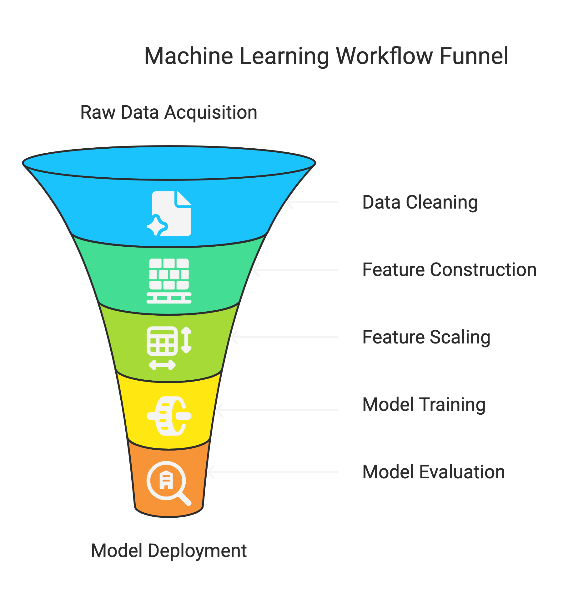
Where It Fits in the ML Workflow:

Here's a simplified view of how feature construction integrates into a typical machine learning pipeline:

• Raw Data Acquisition: Gathering data from various sources.
• Data Cleaning and Preprocessing: Handling missing values, outliers, and inconsistencies.
• Feature Construction: Creating new, informative features from the existing ones (the focus of this discussion).
• Feature Scaling and Transformation: Standardizing or normalizing features to a consistent range.
• Model Selection and Training: Choosing and training a suitable machine learning model.
• Model Evaluation: Assessing the performance of the trained model.
• Deployment and Monitoring: Putting the model into production and tracking its performance.

Tools and Libraries That Help in Feature Construction

Several powerful tools and libraries in Python can significantly facilitate the feature construction process, offering a range of functionalities from basic data manipulation to automated feature engineering.

Using ‘FunctionTransformer’, you can seamlessly integrate custom feature engineering functions into your scikit-learn pipelines. This allows you to apply custom logic to create new features within a structured workflow.

Code example:

import pandas as pd
from sklearn.preprocessing import FunctionTransformer
from sklearn.pipeline import Pipeline
from sklearn.linear_model import LinearRegression

# Custom function to create a feature (e.g., ratio of two columns)
def create_ratio(df):
    df['ratio'] = df['feature1'] / df['feature2']
    return df[['ratio']] # Return a DataFrame

# Sample data
data = {'feature1': [10, 20, 30, 40],
        'feature2': [2, 5, 3, 8],
        'target': [5, 8, 10, 12]}
df = pd.DataFrame(data)

# Create the FunctionTransformer
ratio_transformer = FunctionTransformer(create_ratio)

# Define the pipeline
pipeline = Pipeline([
    ('ratio_feature', ratio_transformer),
    ('linear_regression', LinearRegression())
])

# Train the pipeline
pipeline.fit(df[['feature1', 'feature2']], df['target'])

# Make predictions
predictions = pipeline.predict(df[['feature1', 'feature2']])
print("Predictions:", predictions)

Output:

Predictions: [ 6. 8. 10. 11.]

Explanation:

The code demonstrates how to integrate a custom feature engineering step into a scikit-learn pipeline.

1. create_ratio(df) Function: This function takes a pandas DataFrame, creates a new column named 'ratio' by dividing 'feature1' by 'feature2', and then returns a DataFrame containing only this new 'ratio' feature.
2. FunctionTransformer(create_ratio): Our custom function creates a transformer object. When this transformer is used in a pipeline, the create_ratio function will be applied to the input data.
3. Pipeline(...): A scikit-learn pipeline is defined with two steps:
4. • 'ratio_feature': This step applies our ratio_transformer, creating the new 'ratio' feature.
   • 'linear_regression': This step applies a LinearRegression model. The model will be trained on the original 'feature1' and 'feature2' (implicitly passed through the FunctionTransformer) and the newly created 'ratio' feature.
4. pipeline.fit(...): The pipeline is trained on the 'feature1' and 'feature2' columns of the DataFrame, with 'target' as the target variable. During training, the ratio_transformer first creates the 'ratio' feature, and then the LinearRegression model learns to predict 'target' based on 'feature1', 'feature2', and 'ratio'.
5. predictions = pipeline.predict(...): The trained pipeline is used to predict the same 'feature1' and 'feature2' data. The output [ 6. 8. 10. 11.] shows the predicted values for the 'target' variable based on the learned relationships, including the influence of the constructed 'ratio' feature.

Also Read: Neural Network Architecture: Types, Components & Key Algorithms

Having explored various methods and the integration of feature construction within machine learning pipelines, it's crucial to understand the best practices to follow and the common pitfalls to avoid to ensure the effectiveness and reliability of your engineered features.

Best Practices and Common Pitfalls in Feature Construction

Creating practical features is a blend of art and science. While experimentation is key, adhering to certain best practices can significantly increase the likelihood of constructing valuable features that boost model performance. 

One fundamental principle is to validate new features using rigorous cross-validation or holdout sets to ensure they improve the model's generalization ability rather than just fitting noise in the training data. 

Beyond validation, leveraging feature importance tools like SHAP (Shapley Additive exPlanations) and permutation importance is also insightful. These techniques can help quantify the contribution of each feature to the model's predictions, providing further evidence of a feature's value beyond just cross-validation scores. For instance, a feature that consistently ranks highly important across different validation folds will likely be genuinely informative.

Several other crucial considerations can guide your feature engineering efforts: 

1. Use Domain Knowledge Wherever Possible: Features rooted in a deep understanding of the problem domain often provide stronger and more interpretable signals than those constructed purely through automated or arbitrary transformations. Leverage your expertise to identify relevant relationships and create features that capture these insights.
2. Ensure Temporal Integrity for Time-Based Features: When working with time series data, it's paramount to construct features using only past information. Introducing future data into your feature engineering process (a concept known as "future data leakage") can lead to unrealistically high performance during training but poor generalization to unseen, real-world data.
3. Automate and Log Feature Construction Steps: To maintain consistency, reproducibility, and facilitate collaboration, it's highly recommended to automate your feature construction processes using pipelines or reusable functions. Additionally, meticulously logging the transformations applied and the reasoning behind them can be invaluable for debugging, understanding model behavior, and iterating on your feature engineering strategies.
4. Be Mindful of Feature Redundancy and Multicollinearity: Creating highly correlated features can introduce multicollinearity, destabilizing linear models and making feature importance difficult to interpret. Regularly assess the correlation between your constructed features and consider removing redundant ones.
5. Maintain Feature Interpretability Where Possible: While complex transformations might yield performance gains, strive to create somewhat interpretable features, especially if model understanding is essential. This can aid in debugging, gaining insights, and communicating results effectively.
6. Iterate and Experiment Systematically: Feature construction is often an iterative process. Don't expect to find the optimal set of features on your first attempt. Systematically experiment with different transformations and combinations, always validating their impact on model performance.
7. Consider the Computational Cost of New Features: Some feature construction techniques can significantly increase the dimensionality of your data, leading to higher computational costs for training and inference. Be mindful of this trade-off between potential performance gains and computational efficiency.
8. Document Your Feature Engineering Process: Clearly document the steps involved in creating each feature, including the original features used and the transformations applied. This documentation is crucial for reproducibility and understanding the model.
9. Regularly Review and Refine Features: As your understanding of the data and the problem evolves, revisit your constructed features. Some features that were initially helpful may become less relevant, or new ideas for better features might emerge.

Even though the benefits of engineered features are often touted, a closer examination reveals situations where they can inadvertently create more problems than they solve, as highlighted in the following challenges.

Challenges: When Engineered Features Hurt More Than Help

A critical mistake in feature construction is constructing features using information that would not be available at the time of prediction. This includes using the target variable itself or future data to create features. Such leakage leads to artificially inflated training performance and a model that fails miserably on unseen, real-world data. Some more challenges include: 

• Overfitting with Highly Specific Features: Creating an excessive number of derived features, particularly when working with small datasets, can lead to overfitting. The model might learn intricate patterns specific to the training data, including noise, and consequently perform poorly on new data.
• Redundant or Correlated Features: Constructing features highly similar to existing ones or to each other can introduce multicollinearity. This adds complexity without providing significant new information and can destabilize specific algorithms, making feature importance difficult to interpret.
• Skipping Scaling or Transformation After Construction: Numeric features created through operations like ratios or differences can have drastically different scales or distributions compared to the original features. Failing to apply appropriate scaling or transformations (like standardization or normalization) after feature construction can negatively impact the performance of distance-based models or those sensitive to feature scales.
• Backward Incompatibility: Changes to feature definitions or underlying data sources during model updates can cause inconsistencies and degrade performance in deployed models. Maintaining stable feature pipelines and clear documentation is crucial for production environments.
• Increased Complexity and Reduced Interpretability: Introducing complex engineered features can make the model more complicated to understand and debug. While performance gains are significant, strive to balance accuracy and interpretability, especially in applications where understanding the model's reasoning is crucial.
• Computational Overhead: Constructing many features, or using computationally intensive feature engineering techniques, can significantly increase your models' training and inference time. Consider the trade-off between potential performance improvements and the added computational cost, especially for real-time applications.
• Maintenance and Feature Drift: Engineered features might rely on specific data characteristics or external data sources that could change over time. Monitoring and maintaining these features is essential to prevent performance degradation due to feature drift.
• Ignoring Domain Constraints: Sometimes, seemingly useful engineered features might violate real-world constraints or business rules. Consider your constructed features' practical implications and validity within the specific domain.
• Over-reliance on Automated Feature Engineering: While tools like Featuretools can be powerful, blindly applying automated feature engineering without understanding the generated features can include irrelevant or harmful features. Continually review and validate automatically generated features.

Also read: 15 Key Techniques for Dimensionality Reduction in Machine Learning

As you master the art of feature construction to enhance your machine learning models, consider the exciting possibilities within Generative AI. upGrad's Advanced Certificate Program in Generative AI can equip you with the skills to create novel data and solutions, a powerful complement to insightful feature engineering.

Test Your Understanding of Feature Construction in Machine Learning!

Feature construction is a critical skill in machine learning, enabling the creation of more powerful and insightful models. This short quiz will test your understanding of this tutorial's key concepts and techniques. Take a moment to answer the following ten multiple-choice questions to assess your grasp of feature engineering principles.

1. Which of the following is the primary goal of feature construction? 

a) Selecting the most important features from the original set. 

b) Creating new, potentially more informative features from existing ones. 

c) Scaling numerical features to a standard range. 

d) Encoding categorical features into numerical representations.

2. Forward feature construction is an example of: 

a) Feature construction. 

b) Feature selection. 

c) Feature scaling. 

d) Dimensionality reduction.

3. Creating a 'BMI' feature from 'weight' and 'height' is an example of: 

a) Polynomial features. 

b) Interaction features. 

c) Arithmetic-based features. 

d) Time-based features.

4. Which categorical encoding techniques can be considered a form of feature construction by creating multiple new features? 

a) Label encoding. 

b) Frequency encoding. 

c) One-hot encoding. 

d) Target encoding.

5.Creating 'day of the week' from a timestamp column is an example of: 

a) Lag features. 

b) Rolling window statistics. 

c) Time component extraction. 

d) Text-based feature construction.

6. Which of the following text feature construction techniques considers the importance of a word in a document relative to its frequency across all documents? 

a) N-grams. 

b) Sentiment scoring. 

c) Word embeddings. 

d) TF-IDF.

7. Using cross-validation to assess if a newly constructed feature improves model performance is a: 

a) Common pitfall to avoid. 

b) Best practice in feature construction. 

c) Method for feature scaling. 

d) Technique for handling missing values.

8. Constructing time-based features using future data is an example of: 

a) Feature scaling. 

b) Feature normalization. 

c) Data leakage. 

d) Feature redundancy.

9. Which Python library is specifically designed for automated feature engineering from relational datasets? 

a) pandas. 

b) scikit-learn. 

c) Featuretools. 

d) tsfresh.

10. Integrating a custom feature engineering function into a scikit-learn pipeline can be achieved using: 

a) PolynomialFeatures. 

b) OneHotEncoder. 

c) FunctionTransformer. 

d) StandardScaler.

Also Read: Scikit-learn in Python: Features, Prerequisites, Pros & Cons 

Conclusion

You've now explored the power and nuances of feature construction, a vital skill for any aspiring data scientist. Remember that practical feature engineering is about applying techniques and understanding your data and the problem you're trying to solve. Embrace experimentation, always validate your new features rigorously, and leverage domain knowledge whenever possible to create impactful inputs for your machine learning models.

If you are still struggling to translate raw data into actionable insights and high-performing models, upGrad, in collaboration with Microsoft, offers specialized programs to help you master cutting-edge data analysis and AI skills.

Ready to leverage the latest advancements in generative AI for data analysis? Explore upGrad's specialized program:

• upGrad | Microsoft Gen AI Mastery Certificate for Data Analysis: Master generative AI tools and techniques to enhance your data analysis capabilities and unlock new insights.

Get personalized guidance on the best program for your career goals. Chat with our counselors now! Visit our learning centers across India for in-person guidance and support. Find a center near you!

FAQS

1. What distinguishes feature engineering from feature selection? 

Feature engineering involves creating novel features from the existing dataset through processes like transformation, combination, or the application of domain-specific insights. Conversely, feature selection is about identifying and choosing the most pertinent features already present in the data.

2. Why is feature engineering vital in building machine learning models? 

Effectively engineered features can significantly enhance a machine learning model's performance by supplying more pertinent and informative input variables. This enables the model to discern the underlying patterns within the data better, ultimately leading to greater accuracy and improved out-of-sample prediction.

3. Could you illustrate a basic method for combining features? 

Given 'height' (in meters) and 'weight' (in kilograms), a new feature, 'BMI' (Body Mass Index), can be derived by the formula: weight/(height2). This constructed feature can offer more meaningful insights for specific health-related prediction tasks.

4. In what scenarios would the creation of polynomial features be beneficial? 

Polynomial features are advantageous when a numerical feature exhibits a non-linear relationship with the target variable. For example, if the impact of 'experience' on salary plateaus or even declines after a certain level, incorporating 'experience squared' can help the model represent this more complex relationship.

5. What are interaction features, and what is their utility? 

Interaction features are generated by multiplying two or more existing features. They are valuable for capturing synergistic effects, where the combined influence of several variables yields an outcome that differs from the sum of their individual effects. An example might be the enhanced effectiveness of a marketing email ('sent') during a particular time of the year ('holiday_season').

6. Why is one-hot encoding considered a form of feature construction? 

One-hot encoding transforms a single categorical feature containing multiple categories into a set of new binary (0 or 1) numerical features. Each new feature corresponds to one of the original categories. Thus, it constructs a new, expanded feature space from the initial categorical variable.

7. What is target encoding, and what is a critical consideration for its use?

Target encoding involves replacing each category within a categorical feature with the mean (or another aggregation) of the target variable associated with that category. A crucial point to remember is the potential for data leakage, necessitating robust cross-validation strategies to prevent overfitting.

8. What are some methods for constructing features from time series data? 

Features can be engineered from time series data by extracting temporal components like the day of the week or month, creating lagged variables (past values), and calculating statistics over moving windows (e.g., rolling averages). Encoding cyclical patterns and incorporating holiday information are also standard practices.

9. What are some common challenges or pitfalls to avoid during feature construction? 

Common mistakes include introducing irrelevant noise, creating highly correlated or redundant features, and overfitting the model, particularly when generating numerous features or working with limited data. Furthermore, maintaining the stability of features in production systems is essential.

10. How can the effectiveness of newly engineered features be validated? 

Employing rigorous cross-validation techniques or separate holdout datasets is essential to confirm that new features improve the model's ability to generalize to unseen data, rather than just fitting noise. Examining feature importance scores from relevant tools can provide further insight into a feature's contribution.

11. What are some standard feature construction techniques for text data? 

For text data, common methods include utilizing N-grams (sequences of words), applying TF-IDF to weight word importance, employing sentiment analysis to gauge emotional tone, and using word embeddings to represent words as dense vectors that capture semantic relationships. Dimensionality reduction techniques may be necessary when using N-grams and TF-IDF.