Hierarchical Clustering in Machine Learning: Concepts, Types, and Algorithms

Did you know? Hierarchical clustering analysis has high computational costs. While using a heap can reduce computation time, memory requirements are increased. Both the divisive and agglomerative types of clustering are "greedy," meaning that the algorithm decides which clusters to merge or split by making the locally optimal choice at each stage of the process.

Hierarchical clustering is an unsupervised machine learning algorithm used to group similar data points into clusters. It creates a hierarchy of clusters by either merging small clusters into larger ones (agglomerative) or splitting large clusters into smaller ones (divisive). This method is particularly useful for uncovering complex data relationships.

In this blog, we will dive into the core concepts of hierarchical clustering, explore the differences between agglomerative and divisive types, and examine the algorithms used to implement them. By the end, you’ll have a clear understanding of how hierarchical clustering can enhance your machine learning models.

Explore upGrad's online AI and ML courses to enhance your machine learning skills, master clustering techniques, and improve data analysis. 

What is Hierarchical Clustering in Machine Learning?

Hierarchical clustering is a machine learning technique used to group similar data points into clusters, forming a tree-like structure called a dendrogram. Unlike other clustering methods, it does not require you to specify the number of clusters in advance. 

This method builds clusters step-by-step, either by merging smaller clusters or splitting larger ones, depending on the approach. In this section, we will dive deeper into how hierarchical clustering works, its types, and when to use it effectively.

Machine learning professionals with expertise in clustering techniques, including hierarchical clustering, are in high demand for their ability to analyze and organize complex data. If you're looking to master clustering methods and advance your skills in machine learning, consider these top-rated courses:

• Master's in Artificial Intelligence and Machine Learning
• Executive Diploma in Machine Learning and AI
• Master's Degree in Artificial Intelligence and Data Science

Let us examine how hierarchical clustering fits into unsupervised learning and how it differs from other clustering methods.

How Hierarchical Clustering Fits into Unsupervised Learning?

Hierarchical clustering excels in unsupervised learning by identifying natural groupings in data without the need for labels. It focuses on revealing hidden patterns based on data similarity, allowing you to explore the structure of your dataset without predefined categories. This section will delve into the specifics of how hierarchical clustering operates, its two key types, and practical applications to guide your analysis.

• Exploratory Nature: Ideal when the data structure is not immediately clear and needs flexible exploration.
• Similarity Measures: This technique uses techniques like Euclidean distance to measure similarity, refining clusters for deeper insights into data relationships.
• Unlabeled Data: Unlike supervised learning, hierarchical clustering doesn't require labeled data to predict outcomes, allowing it to work with any unlabelled dataset.
• Applications: Widely used in fields like:
• • Customer Segmentation: Grouping customers based on behaviors or demographics
  • Document Clustering: Organizing text documents into meaningful groups
  • Genomics: Classifying gene expression patterns or biological data

Also Read: Difference Between Supervised and Unsupervised Learning 

Hierarchical Clustering vs. Other Clustering Techniques

Hierarchical clustering differs from other clustering techniques like k-means and DBSCAN in its approach to forming clusters. Unlike k-means, which requires you to define the number of clusters in advance, hierarchical clustering builds a tree-like structure of nested clusters. It also does not rely on the density of data points like DBSCAN, making it more flexible for certain types of data. In this section, we’ll compare hierarchical clustering with other popular methods to help you decide when to use each one.

1. Comparison: K-Means vs. Hierarchical Clustering

2. Comparison: Hierarchical Clustering vs. DBSCAN

upGrad's free Unsupervised Learning: Clustering course will teach you more about clustering techniques. Explore K-Means, Hierarchical Clustering, and practical applications to uncover hidden patterns in unlabelled data.

Also Read: Clustering in Machine Learning: Learn About Different Techniques and Applications

Now that you have understood how hierarchical clustering differs from other clustering methods, let's explore hierarchical clustering algorithms and how they work.

How Does the Hierarchical Clustering Algorithm Work?

Hierarchical clustering works by calculating the similarity or distance between data points or clusters and then progressively merging or splitting them based on this distance. The algorithm continues until all data points are grouped into one cluster or a specified number of clusters is reached. 

Here's how it works:

• Initialization: Start with each data point as its own cluster.
• Iterative Merging/Splitting: In agglomerative clustering, the closest clusters are merged; in divisive clustering, the largest cluster is split.
• Distance Calculation: A linkage method determines how distances between clusters are measured.

Now, let’s break down each step in detail to understand how hierarchical clustering builds its tree structure.

Agglomerative vs. Divisive Approach

In hierarchical clustering, the agglomerative and divisive approaches represent two opposite strategies for forming clusters. Agglomerative starts with individual data points and progressively merges them into larger clusters, while divisive begins with the entire dataset as one cluster and splits it into smaller ones. 

This section will explore the key differences between these approaches, their advantages, and when to use each one for your analysis.

1. Starting Point and Structure of Clusters:

• Agglomerative begins with each data point as its own cluster, progressively merging them into larger groups based on similarity. Think of it like a group of people at a party who start off by mingling in smaller groups and then gradually merge into larger circles as they find common interests.
• Divisive, on the other hand, starts with all data points grouped together and then divides them into smaller, distinct clusters. It’s like starting with a large group and breaking it down into subgroups based on specific characteristics, ensuring that each subgroup is well-defined.

Why it matters: The approach you choose directly affects how your clusters are formed. If your data is naturally hierarchical, agglomerative might give you a smoother progression. Divisive, on the other hand, gives a clearer, top-down separation. However, the time complexity plays a role here—agglomerative clustering generally has a time complexity of O(n^3) due to the need to calculate pairwise distances at each step, making it computationally expensive for large datasets. 

Divisive clustering can have a slightly better time complexity in some cases, but it’s also more resource-intensive in how it splits clusters at each stage.

2. Computational Efficiency and Scalability:

• Agglomerative clustering tends to be more computationally efficient in practice for many datasets. As it builds up clusters gradually, it avoids recalculating distances too often once clusters start to form. However, this efficiency comes with a cost in terms of time complexity, as it requires O(n^2) memory to store the pairwise distances, and as mentioned earlier, it can take up to O(n^3) time in the worst-case scenario.
• Divisive, while often more computationally expensive at each step, can be more scalable for certain types of data. Divisive clustering can have a better worst-case time complexity when dealing with high-dimensional data or when the number of clusters needs to be defined early. However, its efficiency depends largely on how well it splits the initial cluster.

Why it matters: If your dataset is large or time-sensitive, the time complexity of these methods becomes crucial. Agglomerative clustering might be the go-to for smaller datasets, but divisive clustering could be more effective for datasets where a defined split is needed early on. Understanding how time complexity affects performance helps you select the method that balances speed with accuracy.

3. Handling Outliers and Noise:

• Agglomerative clustering is more prone to merging noisy data points early in the process because it focuses on merging the closest clusters, including outliers in the process. This can lead to skewed or distorted results if the data contains a lot of noise.
• Divisive, on the other hand, is less likely to group outliers into the main clusters. Since divisive clustering begins by considering the entire dataset as one cluster, it can more effectively separate outliers from meaningful data by splitting them off early in the process.

Why it matters: In real-world scenarios, noisy data can distort your results. If your dataset is noisy or includes outliers that you don’t want affecting the clusters, divisive clustering may help better isolate these points. However, agglomerative clustering’s tendency to merge smaller groups quickly can lead to less clean segmentation unless pre-processing steps are taken.

4. Cluster Cohesion and Separation:

• Agglomerative tends to create more fluid clusters where the members within a cluster are closely related. This is ideal for situations where smaller, more cohesive groups should be formed gradually. However, as the complexity increases, the method can sometimes merge less relevant clusters due to its progressive merging nature.
• Divisive produces clearer, well-separated clusters early in the process, which can be beneficial when you need distinct categories. It works well when you have data that should naturally divide into large segments with little overlap.

Why it matters: The choice of approach impacts the separation and cohesion of your clusters. Divisive clustering’s top-down method creates clearer divisions, while agglomerative clustering’s gradual merging forms more natural, tightly-knit groups. Keep in mind that divisive clustering, with its distinct separations, may require more detailed calculations and take more time.

5. Practical Use Case:

• Agglomerative: Let’s say you are analyzing customer behavior in an e-commerce store. You start by categorizing each user’s activity and gradually group them based on similarities, such as purchasing habits. Over time, smaller clusters like “frequent buyers” or “browsers” merge into broader categories like “loyal customers” or “seasonal shoppers.”
• Divisive: Now, let’s imagine you want to create customer segments based on high-level categories right away, such as separating “premium customers” from “basic customers.” Divisive clustering starts by dividing the entire customer base into these broad segments and then breaks them down into smaller, more specific subgroups.

Why it matters: Depending on your business needs, you might prefer the organic growth of clusters in agglomerative clustering or the clear-cut divisions of divisive clustering. When considering time complexity, though, remember that large datasets will be computationally expensive for agglomerative clustering, which might affect real-time customer segmentation.

6. Real-world Application:

• Agglomerative: You are tasked with segmenting documents for a research project. The agglomerative method allows you to start by treating each document as a distinct topic, and as you group them by shared themes, you can gradually form meaningful categories, such as “scientific papers” or “literature reviews.”
• Divisive: For a more structured dataset, like customer reviews, divisive clustering could immediately divide the reviews into clear, high-level categories like “positive” and “negative” before refining them into more specific groups like “product quality” or “customer service.”\

Why it matters: The right approach helps you create meaningful, actionable insights. Agglomerative clustering offers flexibility and nuance in clustering, but divisive clustering provides clarity and speed in separating large, diverse datasets.

Conceptual Example: Agglomerative vs. Divisive

In this section, you’ll see a conceptual example comparing the agglomerative and divisive approaches in hierarchical clustering. You’ll understand how agglomerative clustering builds clusters from the bottom up by merging smaller groups, while divisive clustering works from the top down, starting with one large group and splitting it into smaller ones. 

This example will help you visualize the practical differences and guide you in choosing the right approach for your data.

Now that we’ve compared Agglomerative and Divisive clustering approaches, let's focus on the step-by-step process of performing Agglomerative Hierarchical Clustering. This will provide a clear, practical guide for applying this method to your data.

How to Perform Agglomerative Hierarchical Clustering Step by Step?

To perform agglomerative hierarchical clustering step by step, you start by calculating the distance between each data point. Then, you progressively merge the closest pairs into clusters, repeating this process until all points are grouped into one. This guide will walk you through each stage, providing clarity on how to apply this method effectively using available tools.

Step 1: Start with each data point as its cluster

At the beginning, every data point in the dataset is treated as its own cluster. If you have a dataset with 10 points, you will have 10 clusters to begin with.

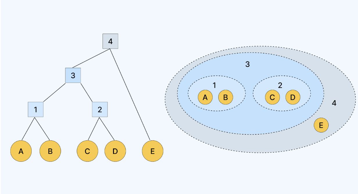
• Example: Consider five data points: A, B, C, D, and E. Initially, these are all their clusters:{A}, {B}, {C}, {D}, {E}

Step 2: Compute the pairwise distances between all clusters

To determine which clusters to merge, you need to calculate the distance between all pairs of clusters. The most common distance metric used is Euclidean distance, though others like Manhattan or Cosine distance can be used depending on the problem.

• Example: If you are working with two points, P1 (1, 2) and P2 (2, 3), you would calculate the Euclidean distance between them as follows:

Step 3: Merge the two closest clusters

Once the pairwise distances are computed, you merge the two clusters with the smallest distance, reducing the number of clusters by one.

• Example: If the distance between clusters {A} and {B} is the smallest, then they will be merged into a single cluster: {A, B}, {C}, {D}, {E}

Also Read: What is Cluster Analysis in Data Mining? Methods, Benefits, and More

Step 4: Update the distance matrix

After merging the two clusters, the next step is to update the distance matrix, which now includes the newly formed cluster. The distance between the new cluster and other clusters needs to be calculated. This is typically done using one of several linkage methods:

• Single linkage: The distance between two clusters is the shortest distance between any two points from the two clusters.
• Complete linkage: The distance between two clusters is the longest distance between any two points from the two clusters.
• Average linkage: The distance is the average distance between all pairs of points from the two clusters.
• Example: If {A, B} were merged, you now need to calculate the distance between {A, B} and other clusters like {C}, {D}, and {E}. This can be done using single or complete linkage.

Step 5: Repeat until one cluster remains

The process of calculating pairwise distances, merging the closest clusters, and updating the distance matrix is repeated iteratively until all the data points are merged into a single cluster or until a desired number of clusters is reached.

• Example: After the first merge, you would have:{A, B}, {C}, {D}, {E}

Next, you would calculate the distances between these clusters, merge the closest pair, and continue until you are left with a single cluster: {A, B, C, D, E}

Summary of Agglomerative Hierarchical Clustering Steps:

1. Initialize: Treat each data point as its cluster.
2. Calculate Pairwise Distances: Use a distance metric like Euclidean distance.
3. Merge Closest Clusters: Combine the two clusters that are closest to each other.
4. Update Distance Matrix: Recalculate distances based on the new clusters.
5. Repeat: Continue merging and updating distances until all data points are in one cluster.

Visual Representation:

To better understand these steps, look at the following:

Ready to take your data science skills to the next level? The upGrad's Data Science Master’s Degree offers a comprehensive pathway to mastering key concepts like agglomerative hierarchical clustering. Enroll today to deepen your expertise and unlock new opportunities in the field of data science!

Also Read: What is Clustering in Machine Learning and Different Types of Clustering Methods

Now that you know what agglomerative clustering is and how it differs from the divisive approach, let's examine the types of hierarchical clustering and their linkage methods.

Types of Hierarchical Clustering and Linkage Methods

In hierarchical clustering, you can choose between two main types: agglomerative (bottom-up) and divisive (top-down). Each type relies on linkage methods such as single, complete, average, and Ward’s method to determine how clusters are formed based on distance between data points or clusters. 

Understanding these methods helps you select the most appropriate approach for your dataset. The table below outlines these types and their key characteristics.

Here’s a summary of the different distance metrics and linkage methods used in hierarchical clustering:

Now, let’s look at the different linkage methods and how each one affects the clustering process.

Common Linkage Criteria

Linkage criteria determine how the distance between clusters is calculated during hierarchical clustering. Common methods include single, complete, and average linkage, each measuring distances differently to influence how clusters are merged. This section will explore these criteria, helping you understand their impact on the final clustering result and when to use each one.

Below are the most commonly used linkage methods. 

1. Single Linkage

Single linkage (also known as nearest point linkage) calculates the distance between two clusters based on the closest pair of points between them. In essence, it uses the minimum distance between clusters to decide whether to merge them. 

Single linkage is prone to producing "chained" clusters, where data points may be loosely connected and form elongated, irregular shapes. It's often described as "floppy" because a single distant outlier can cause clusters to merge unexpectedly.

• How it works: The distance between two clusters is the smallest distance between any two points, one from each cluster.
• Example: Imagine we have two clusters, A = 1, 2, and B = 5, 6. In single linkage, we calculate the distance between the closest points in A and B (e.g., 2 and 5), which is 3. If this distance is the smallest among all possible distances, these clusters will be merged.
• When to use:
• • Use single linkage when you expect elongated or chain-like clusters.
  • This is ideal for cases where there may be outliers in the data, but you still want to keep them grouped with the rest.

2. Complete Linkage

Complete linkage (or farthest point linkage) calculates the distance between two clusters based on the furthest pair of points, one from each cluster. This results in more compact clusters than single linkage because it's less sensitive to individual outliers. Complete linkage ensures that all points within a cluster are close to each other, which helps in avoiding the formation of elongated clusters.

• How it works: The distance between two clusters is defined by the maximum distance between any two points from the two clusters.
• Example: For clusters A = {1, 2} and B = {5, 6}, the distance between them would be the maximum distance between all pairs, such as the distance between 1 and 6, or 2 and 5, which would be 5.
• When to use:
• • Choose complete linkage when you need compact, spherical clusters.
  • Best for data where you want tight clusters with minimal variation within them.

3. Average Linkage

Average linkage calculates the distance between two clusters by averaging the pairwise distances between all points in the first cluster and all points in the second cluster. This method strikes a middle ground between single and complete linkage and is useful when you expect clusters to be fairly compact, but with some variation in their shape.

• How it works: The distance between two clusters is the average of the distances between all pairs of points (one from each cluster).
• Example: For clusters A = {1, 2} and B = {5, 6}, the distance between the clusters would be the average of all pairwise distances:
• When to use:
• • Use average linkage when the data does not have a clear elongated or tight structure.
  • Ideal for general clustering tasks where you want to balance between compactness and flexibility.

4. Ward's Method

Ward's method minimizes the within-cluster variance by merging clusters that result in the smallest increase in the total variance of the data. It is often considered the most efficient linkage method when you expect spherical clusters because it leads to balanced and tight clusters. Unlike the other methods, Ward's method is based on minimizing the variance rather than simply measuring distances.

• How it works:

The algorithm calculates the total sum of squared differences (variance) within each cluster and merges the two clusters that result in the least increase in this variance.

• Example: Suppose clusters A and B are merged. The new cluster's variance is calculated, and the increase in variance is compared with the increase from other potential merges. If merging A and B results in the smallest increase, they will be merged.
• When to use:
• • Ward's method is highly effective when you have well-separated, spherical clusters.
  • This method is particularly useful when minimizing the variability within each cluster is important.

Euclidean Distance Formula:

Ward's method typically relies on the Euclidean distance to measure the similarity between clusters. Euclidean distance is the most common way to calculate distance in continuous space, and it's used to determine how "close" or "distant" data points or clusters are.

• Euclidean Distance Formula for two points P(x_1, y_1) and Q(x_2, y_2) in a 2-dimensional space is:

• In higher dimensions, the formula generalizes to:

Where x_i and y_i are the coordinates of the points in an n-dimensional space.

Ward's method uses this distance to calculate the initial "distance" between clusters, and as clusters are merged, the centroid of the new cluster is recalculated.

Choosing the Right Linkage Based on Data Structure

Choosing the right linkage criteria depends on the structure of your data and the type of clusters you want to form. For instance, single linkage works well with elongated clusters, while complete linkage is better for compact, well-separated clusters. This section will guide you in selecting the most appropriate linkage method based on the characteristics of your dataset and clustering goals.

Below is a guide to help you select the appropriate linkage based on your data's structure:

Are you a full-stack developer wanting to integrate AI into your Python programming workflow? upGrad's AI-Driven Full-Stack Development bootcamp can help you. You'll learn how to build AI-powered software using OpenAI, GitHub Copilot, Bolt AI & more.

Also Read: Hierarchical Clustering in Python [Concepts and Analysis] 

Now that we've covered the types of hierarchical clustering and linkage methods, let's explore the tools and libraries to implement them in your machine learning projects.

Tools and Libraries to Implement Hierarchical Clustering in ML

To apply hierarchical clustering in machine learning, you can use libraries like Scikit-learn, SciPy, and Seaborn, each offering specific functions for building, visualizing, and analyzing clusters. 

These tools support various linkage methods and distance metrics, making them adaptable to different use cases. The list below highlights the key features and use cases of each library.

1. Using Scikit-Learn and SciPy

Using Scikit-Learn and SciPy allows you to efficiently implement hierarchical clustering with just a few lines of code. Scikit-Learn provides a user-friendly interface for clustering tasks, while SciPy offers advanced linkage methods and distance calculations. This section will walk you through how to use these libraries to perform hierarchical clustering, making the process straightforward and accessible.

Sample Code Using Agglomerative Clustering and Linkage + Dendrogram

Here's a practical example of how to perform hierarchical clustering using Scikit-learn for the clustering and SciPy for visualizing the results with a dendrogram.

# Import necessary libraries
import numpy as np
import matplotlib.pyplot as plt
from sklearn.cluster import AgglomerativeClustering
From scipy.cluster.hierarchy import dendrogram, linkage

# Sample data
X = np.array([[1, 2], [3, 3], [6, 5], [8, 8], [1, 1], [7, 6]])

# Agglomerative Clustering using Scikit-learn
agg_clust = AgglomerativeClustering(n_clusters=2, affinity='euclidean', linkage='ward')
agg_clust.fit(X)

# Plotting the Dendrogram using SciPy
Z = linkage(X, 'ward')
plt.figure(figsize=(10, 7))
dendrogram(Z)
plt.title("Dendrogram")
plt.xlabel("Data Points")
plt.ylabel("Euclidean Distance")
plt.show()

• Explanation:
• • Agglomerative Clustering: This method from Scikit-learn performs the clustering. We specify the number of clusters (2 in this case), the distance metric (Euclidean), and the linkage method (Ward).
  • Linkage: The linkage function in SciPy calculates the hierarchical clustering linkage matrix, which is needed to plot the dendrogram.
  • Dendrogram: The dendrogram function visualizes the merging process of clusters, showing the distances at which clusters are merged.
• Expected Output:

2. Visualizing Clusters with Dendrograms

Dendrograms are a powerful way to visualize the results of hierarchical clustering, showing how clusters are merged at each step. By plotting the hierarchical structure, you can easily determine the optimal number of clusters and understand the relationships between them. This section will guide you through the process of creating and interpreting dendrograms, helping you gain deeper insights into your clustering results.

Steps to Plot Dendrograms:

1. Calculate the linkage matrix: Use SciPy's linkage function to compute the distances between clusters.
2. Plot the dendrogram: Use SciPy's dendrogram function to create a visual representation of the hierarchical clustering.

• Interpretation:
• • Vertical lines in the dendrogram represent the distance at which clusters are merged. The higher the line, the more dissimilar the two clusters are.
  • Horizontal lines represent the clusters at each stage. By cutting the dendrogram at a specific height, you can define the number of clusters that best suit your analysis.

Example of Interpreting a Dendrogram

Consider the following example where we visualize the hierarchical clustering results for a set of data points. By analyzing the dendrogram, we can determine the optimal number of clusters by identifying where the large vertical distances occur. If there is a large vertical gap between two clusters, it suggests a significant difference between them.

Role of Dendrograms in Agglomerative Hierarchical Clustering

Dendrograms play a keyl role in agglomerative hierarchical clustering by visually representing how clusters are merged at each step. They help you trace the progression of clustering and identify the most suitable point to cut the tree for optimal cluster formation. In this section, you’ll learn how to interpret dendrograms and use them to refine your clustering decisions.

How Dendrograms Help Determine the Optimal Number of Clusters?

• The main advantage of dendrograms is that they help you decide the number of clusters by cutting the tree at the most meaningful point.
• The height at which you cut the dendrogram determines the number of clusters. Cutting higher means fewer clusters, while cutting lower means more clusters.

Reading Vertical and Horizontal Relationships

• Vertical distances (linkage distance) represent the dissimilarity between clusters when they merge. A large vertical distance indicates that the clusters being merged are very different from each other.
• Horizontal relationships show which clusters are being merged at each step and their relative positions.

Using SciPy's dendrogram for Plotting

The scipy.cluster.hierarchy.dendrogram function allows you to plot the dendrogram easily. By passing the linkage matrix from the linkage function, you can generate a plot that shows the merging sequence of your data points.

Visualizing and Interpreting Cluster Hierarchies

Visualizing and interpreting cluster hierarchies helps you understand the relationships between data points at different levels of clustering. By examining dendrograms or other visual tools, you can easily identify natural groupings and determine the optimal number of clusters. This section will show you how to effectively analyze cluster hierarchies, enabling you to make data-driven decisions on cluster selection.

Example:

# Sample dataset
X = np.array([[2, 4], [1, 1], [6, 8], [7, 5], [5, 4]])

# Compute linkage matrix
Z = linkage(X, 'ward')

# Plot a dendrogram
plt.figure(figsize=(10, 7))
dendrogram(Z)
plt.title("Dendrogram Example")
plt.xlabel("Data Points")
plt.ylabel("Linkage Distance")
plt.show()

Expected Output:

Evaluating Hierarchical Clustering Output

Evaluating hierarchical clustering output allows you to assess the effectiveness of the clusters formed by your algorithm. You’ll look at metrics like silhouette score, cluster cohesion, and separation to determine how well the data points are grouped. In this section, we will dive into specific evaluation techniques, providing you with the tools to validate your clustering results.

Internal Validation Metrics

• Cophenetic Correlation Coefficient (CCC): This metric measures how well the hierarchical clustering results preserve the distances between data points. A higher CCC indicates that the clustering process is well-aligned with the actual distances between points.
• Silhouette Score: This score evaluates how well-separated the clusters are. A higher silhouette score suggests that the clusters are well-defined and distinct.

Challenges in Evaluation

A major challenge in evaluating hierarchical clustering is that there is no ground truth in unsupervised learning. Since hierarchical clustering doesn't have predefined labels, you cannot directly compare the clusters against any correct answer.

• Example:
• • In customer segmentation, you may have no predefined groups, and choosing the right number of clusters depends on how useful the clusters are for business analysis, not just statistical validation.

Decoding what drives customer action can be easy with upGrad's free Introduction to Consumer Behavior course. You will explore the psychology behind purchase decisions, discover proven behavior models, and learn how leading brands influence buying habits.

Also Read: Understanding the Concept of Hierarchical Clustering in Data Analysis: Functions, Types & Steps 

Now that we have understood the Tools and Libraries for Implementing Hierarchical Clustering in ML, let's explore hierarchical clustering in data mining applications.

Hierarchical Clustering in Data Mining Applications

You can apply hierarchical clustering in data mining to uncover hidden patterns in areas like customer segmentation, document classification, and gene expression analysis. Its ability to build nested clusters makes it suitable for exploring complex, multi-level data relationships. The examples below illustrate how it's used across different domains.

Let's explore some key applications of hierarchical clustering in real-world scenarios.

1. Customer Segmentation

Customer segmentation is the process of dividing your customer base into distinct groups based on shared characteristics such as behavior, demographics, or preferences. This allows you to tailor marketing strategies and improve targeting. In this section, we’ll explore how hierarchical clustering can be used for effective customer segmentation, providing practical insights for applying this method.

• How it works: Hierarchical clustering groups customers based on similarities in their behaviors, preferences, or demographics. The resulting clusters help identify distinct customer profiles that can be targeted with tailored strategies.
• Use Case:
• • In the retail industry, a company can use hierarchical clustering to segment customers based on their purchasing history. For instance, they may identify segments like frequent buyers, seasonal buyers, and discount-driven shoppers. This segmentation helps the company design specific marketing campaigns, such as loyalty programs for frequent buyers or promotions targeted at seasonal shoppers.
• Key Benefits:
• • Helps businesses understand customer behavior in depth.
  • Enables more targeted marketing strategies based on customer clusters.

2. Document or Text Clustering

Document or text clustering is the process of grouping similar documents or texts based on content, helping to identify themes or topics within large datasets. This method is useful for organizing, summarizing, and retrieving relevant information. In this section, we will show you how hierarchical clustering can be applied to text data, making it easier to analyze and categorize documents effectively.

• How it works: Hierarchical clustering organizes documents or text data based on similarity measures like TF-IDF (Term Frequency-Inverse Document Frequency) or cosine similarity. This method allows grouping documents into clusters that share similar topics or themes.
• Use Case:
• • A news aggregation platform might use hierarchical clustering to automatically group articles based on topics such as sports, politics, or technology. By visualizing the relationships between different articles in a dendrogram, the platform can recommend content to users based on their preferred topics.
• Key Benefits:
• • Automatically categorizes large volumes of unstructured text data.
  • Improves search efficiency and content recommendation systems.

3. Bioinformatics and Gene Expression Analysis

Bioinformatics and gene expression analysis involves using clustering techniques to analyze gene data and uncover patterns in gene expression across different conditions or samples. This helps in identifying relationships between genes and understanding biological processes. In this section, we’ll explore how hierarchical clustering is applied in bioinformatics to analyze gene expression data, offering insights into its practical use for genetic research.

• How it works: Hierarchical clustering in bioinformatics typically uses Euclidean distance or Pearson correlation to assess the similarity between gene expression profiles. Genes with similar expression patterns are grouped, allowing researchers to identify gene clusters that may be related to specific biological processes or conditions.
• Use Case:
• • In cancer research, hierarchical clustering can be used to identify genes that behave similarly across different cancer types. For example, researchers might use clustering to find gene signatures specific to breast cancer or lung cancer, which can help identify potential biomarkers for early diagnosis or targeted treatments.
• Key Benefits:
• • Helps in identifying meaningful patterns in complex biological data.
  • Aids in understanding gene functions and disease mechanisms, leading to potential advancements in personalized medicine.

Now let's check your understanding with a short quiz. Please complete the quiz carefully before looking at the answers.

Quiz to Test Your Knowledge on Hierarchical Clustering in Machine Learning

This quiz lets you check your understanding of key concepts in hierarchical clustering, including types, linkage methods, and real-world applications. You’ll answer multiple-choice questions that reinforce what you’ve learned. Use the quiz below to evaluate your grasp of the material.

Test your knowledge now!

1. What does hierarchical clustering aim to achieve in machine learning?

• A) Classify data into pre-defined categories
• B) Group similar data points into clusters
• C) Reduce the number of features in the dataset
• D) Increase the dimensionality of the data

2. Which of the following is a key characteristic of hierarchical clustering?

• A) It requires the number of clusters to be predefined
• B) It produces a tree-like structure called a dendrogram
• C) It only works with labeled data
• D) It uses a flat clustering method for grouping data

3. Which linkage method calculates the distance based on the closest pair of points from two clusters?

• A) Single linkage
• B) Complete linkage
• C) Average linkage
• D) Ward's method

4. What is the main drawback of single-linkage clustering?

• A) It tends to produce compact, spherical clusters
• B) It is highly sensitive to noise and outliers
• C) It always results in balanced clusters
• D) It cannot handle large datasets

5. In which situation is complete linkage clustering most effective?

• A) When you expect elongated or irregularly shaped clusters
• B) When you need compact, tightly bound clusters
• C) When the data is noisy and contains outliers
• D) When clusters are unevenly distributed

6. What does Ward's method minimize when merging clusters?

• A) Linkage distance
• B) Within-cluster variance
• C) Outlier presence
• D) Number of clusters

7. Which of the following is the correct representation of a dendrogram?

• A) A graph showing the performance of the algorithm over time
• B) A tree-like diagram showing the sequence of cluster merges
• C) A scatter plot with data points colored by cluster
• D) A histogram displaying the frequency distribution of data

8. How can the optimal number of clusters be determined using a dendrogram?

• A) By counting the number of clusters in the dataset
• B) By cutting the tree at a specific vertical height
• C) By calculating the silhouette score
• D) By applying K-means after hierarchical clustering

9. What is a common application of hierarchical clustering in customer segmentation?

• A) To classify customers into predefined categories
• B) To group customers based on their purchasing behavior
• C) To find the optimal number of products for sale
• D) To identify customer preferences for specific brands

10. In bioinformatics, hierarchical clustering is often used to group genes based on their:

• A) Color intensity
• B) Gene expression levels across different conditions
• C) Protein sequence similarity
• D) Geographical distribution

Answers:

B) Group similar data points into clusters

1. B) It produces a tree-like structure called a dendrogram
2. A) Single linkage
3. B) It is highly sensitive to noise and outliers
4. B) When you need compact, tightly bound clusters
5. B) Within-cluster variance
6. B) A tree-like diagram showing the sequence of cluster merges
7. B) By cutting the tree at a specific vertical height
8. B) To group customers based on their purchasing behavior
9. B) Gene expression levels across different conditions

Upskill with upGrad to Stay Ahead of Industry Trends! 

By now, you’ve learned how hierarchical clustering works, the types and linkage methods involved, and where it's applied in real-world scenarios. Use this knowledge to evaluate clustering problems more confidently and choose the right technique based on your data structure and analysis goals. Applying these insights can significantly improve your approach to unsupervised learning tasks.

If you’re looking to deepen your expertise but feel unsure about the next step or how to bridge skill gaps, upGrad offers structured, mentor-guided programs tailored to real industry demands. These courses not only build your technical foundation but also help you stay aligned with evolving machine learning trends for long-term career growth.

While the course covered in the article can significantly improve your knowledge, here are some additional free courses from upGrad to facilitate your continued learning:

• Hypothesis Testing
• Unsupervised Learning: Clustering
• Logistic Regression for Beginners
• Linear Regression - Step by Step Guide
• Introduction to Natural Language Processing

You can also get personalized career counseling with upGrad to guide your career path, or visit your nearest upGrad center and start hands-on training today! 

FAQs 

1. What is the main difference between agglomerative and divisive hierarchical clustering?

Agglomerative clustering starts with each data point as its own cluster and progressively merges them based on similarity, while divisive clustering starts with all data points in one cluster and progressively splits them into smaller clusters. Agglomerative is a bottom-up approach, and divisive is a top-down approach.

2. How does hierarchical clustering handle unlabelled data?

Hierarchical clustering is particularly useful in unsupervised learning because it doesn’t require labeled data. It works by grouping similar data points together based on their inherent characteristics, which is ideal when there are no predefined categories.

3. Why is the time complexity important when choosing between agglomerative and divisive clustering?

Time complexity is a key factor because agglomerative clustering can become computationally expensive with large datasets, as it requires calculating pairwise distances repeatedly, leading to O(n^3) complexity. Divisive clustering can sometimes be more efficient in handling large, high-dimensional datasets but may still be resource-intensive depending on the split strategy.

4. When should I use complete linkage over single linkage in hierarchical clustering?

Use complete linkage when you need compact and well-separated clusters. It ensures that the clusters being merged are tightly bound, making it less sensitive to outliers. On the other hand, single linkage can result in elongated or “chained” clusters, which are not ideal for tight groupings.

5. What are the practical applications of hierarchical clustering in customer segmentation?

Hierarchical clustering helps in grouping customers based on purchasing behaviors, demographics, or engagement. It enables businesses to identify customer segments such as frequent buyers or seasonal shoppers, which can then be targeted with specific marketing strategies or loyalty programs.

6. How can I interpret a dendrogram to determine the optimal number of clusters?

A dendrogram helps determine the optimal number of clusters by cutting the tree at a specific height. The larger the vertical distance between merges, the more distinct the clusters are. By selecting the point where these large vertical gaps appear, you can identify an appropriate number of clusters.

7. What are the strengths of using Ward’s method in hierarchical clustering?

Ward’s method minimizes the within-cluster variance, making it ideal for creating compact, spherical clusters with minimal internal variability. It is particularly effective when clusters are well-separated and you want to ensure that the clustering result is balanced and tight.

8. How does hierarchical clustering compare to DBSCAN?

While DBSCAN focuses on grouping data based on density and can handle arbitrary shapes, hierarchical clustering focuses on forming clusters based on similarity and produces a tree-like structure (dendrogram). Hierarchical clustering is better suited when you need to explore multi-level structures, while DBSCAN is ideal for identifying clusters in noisy, unevenly distributed data.

9. Can hierarchical clustering be used with large datasets?

Hierarchical clustering can be computationally expensive, especially for large datasets, as it requires calculating pairwise distances between every data point. For very large datasets, alternative clustering methods like k-means or DBSCAN might be more practical, but if you’re working with smaller or moderately sized datasets, hierarchical clustering can be quite effective.

10. What distance metrics are commonly used in hierarchical clustering?

Common distance metrics include Euclidean distance, which calculates straight-line distance between data points, Manhattan distance, which sums the absolute differences of coordinates, and cosine distance, which measures the angle between two vectors, especially used in text clustering. The choice of distance metric depends on the type of data being analyzed.

11. How can I visualize hierarchical clustering results effectively?

The best way to visualize hierarchical clustering results is by using a dendrogram, a tree-like diagram that shows how clusters are merged or split. It helps in understanding the relationships between clusters and determining the optimal number of clusters by cutting the dendrogram at a meaningful point. Tools like SciPy’s dendrogram function can assist in creating these visualizations.