Standard Deviation Formula: Definition, Calculation & Examples

Standard deviation in machine learning models is a statistical measure that represents the amount of variation or dispersion in a dataset. It shows how spread out data points are from the mean, which is essential for understanding data variability and ensuring accurate model performance. Understanding this variability helps identify patterns, detect anomalies, and improve feature selection in ML across diverse domains like finance, healthcare, and marketing.

In this guide, you’ll learn what standard deviation ML is, how to calculate and interpret it, and why it’s vital for feature scaling and anomaly detection. We will also explore its practical challenges and limitations to provide a well-rounded understanding of this core concept.

Want to learn how the standard deviation in machine learning models enhances performance and accuracy? upGrad’s Artificial Intelligence & Machine Learning - AI ML Courses backed by 1,000+ industry partners and boosting salaries by 51% on average, equip you with the skills to advance your career and master ML techniques.

Understanding Standard Deviation ML: Definition and Significance

In machine learning, statistics are essential for interpreting, processing, and analyzing data. One key statistical measure is the standard deviation, which quantifies the variability or spread of data points within a dataset. This measure indicates how much individual data points differ from the mean and is especially important when working with datasets of varying sizes, distributions, or noise levels. Below is the standard deviation formula:

Where:

• σ represents the standard deviation
• Σ indicates the summation
• x stands for each individual data value
• μ is the mean (average) of the dataset
• N is the total number of values in the dataset

A high standard deviation means the data points are widely dispersed, while a low standard deviation indicates that the data points are clustered around the mean.

Example Use Case: In K-Nearest Neighbors (KNN), features with high variance can disproportionately influence distance calculations, potentially skewing the model’s predictions if data isn’t properly scaled or normalized using standard deviation-based methods.

By measuring variability using standard deviation, you can identify unstable features, normalize feature scales, and detect anomalies, which are key steps that help optimize machine learning models and improve prediction accuracy.

Want to enhance your understanding of key ML concepts like standard deviation and boost your career? Check out these courses to gain the knowledge and hands-on experience needed to handle huge data and improve your ML models confidently:

• Executive Diploma in Machine Learning and AI with IIIT-B
• Master’s Degree in Artificial Intelligence and Data Science
• Generative AI Mastery Certificate for Software Development

Understanding the calculation process of standard deviation helps you appreciate its role in data analysis. Lets break down the steps involved in measuring how spread out your data points are from the average.

How to Calculate Standard Deviation: Step-by-Step Process

Calculating standard deviation involves measuring the average distance of data points from the mean (average) using the standard deviation formula. Below is a step-by-step process that clearly and accurately quantifies data variability.

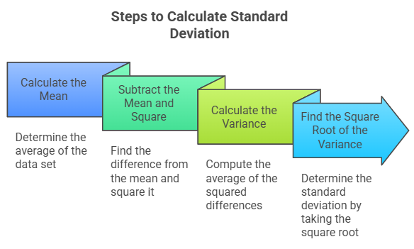
Step 1: Calculate the Mean

To begin, find the mean of the dataset. The mean is the sum of all data points divided by the number of points in the dataset.

Formula:

Where:

• xi represents each individual data point.
• N is the total number of data points.

This step helps you determine the dataset's central value (average), which is crucial for understanding overall trends and for further statistical calculations.

Step 2: Subtract the Mean and Square the Result

For each data point, subtract the mean (calculated in Step 1), then square the result. This emphasizes larger gaps from the mean, ensuring that both positive and negative deviations contribute equally to the overall spread.

Formula:

Where μ is the mean.

This step measures how far each data point is from the mean. Squaring the differences removes negative signs and gives more weight to larger deviations, helping to understand the variability in the dataset.

Step 3: Calculate the Variance

Variance measures how much the data points in a set differ from the mean on average. It’s calculated as the average of the squared differences between each data point and the mean, providing a numerical value that reflects the spread or dispersion of the data. There are two main formulas for variance, depending on whether you’re analyzing an entire population or just a sample:

• Population Variance (σ²): Use this formula when your data includes every member of the entire group or population you want to analyze. This means you have complete information about the whole set you are interested in.

Formula :

Sample Variance (s²): Use this formula when your data represents only a subset or sample from a larger population. Since you’re working with incomplete information, this formula adjusts by dividing by N-1, correcting bias through Bessel’s correction to provide a more accurate estimate.

Formula :

Since training data in machine learning is usually a sample of the overall population, models rely on sample variance to accurately estimate data variability. This helps improve generalization and performance on unseen data.

Step 4: Find the Square Root of the Variance

Finally, the standard deviation is the square root of the variance. This step converts the variance back to the original units of the data, making the measure of spread easier to interpret.

Formula:

This standard deviation formula is crucial for understanding data variability. Having a hands-on understanding of how standard deviation is calculated helps in machine learning by improving preprocessing steps like feature scaling and normalization. It also aids in interpretability model variance and uncertainty in predictions, ultimately enhancing model tuning and performance evaluation.

To make the process easier to understand, let’s break down a practical example using a simple dataset.

Example of Standard Deviation Calculation: Suppose you have the following dataset representing the test scores of 5 students:

Step 1: Calculate the Mean

This step finds the average score, which serves as a reference point to measure deviation from the center.

Step 2: Subtract the Mean and Square the Result

Here, you measure how far each data point is from the mean. By squaring these differences, you remove negative signs and emphasize larger gaps, helping you accurately capture the spread of your data.

Step 3: Calculate the Variance

In this step, variance gives us the average of the squared differences from the mean. It quantifies how spread out or clustered the data is.

Step 4: Find the Square Root of the Variance

Finally, we take the square root of the variance to return to the original units. This value is the standard deviation, which tells us how much the scores typically differ from the mean.

Interpretation: A standard deviation of about 3.41 means that, on average, each test score differs from the mean score of 90 by roughly 3.41 points. In modeling, a similar concept applies when analyzing residuals, the differences between predicted and actual values. The standard deviation of residuals helps measure model accuracy and consistency.

Additionally, during cross-validation, variability in performance metrics across folds reflects how stable and generalizable the model is. Understanding this variability through standard deviation guides improvements and ensures robust predictions.

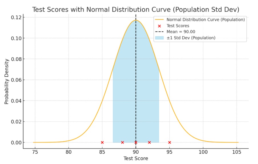
To better understand the spread of the test scores, we can visualize the data on a normal distribution curve with the mean and standard deviation.

• The mean (90) is marked by the dashed black line.
• The red dots represent the actual test scores: 85, 90, 92, 88, 95.
• The blue shaded region represents ±1 standard deviation (3.41) from the mean, covering approximately 86.59 to 93.41.
• Most of the scores fall within this range, indicating the scores are fairly consistent and close to the mean. The distribution is relatively normal.

Looking to build your expertise in key ML concepts like standard deviation and beyond? Gain comprehensive knowledge of Deep Learning, Generative AI, NLP, and more with upGrad’s Executive Programme in Generative AI for Leaders. Elevate your skills and prepare for impactful careers in AI and data science.

For statistical measures like standard deviation, efficiency and accuracy are key. To save time and reduce errors, let’s explore software tools designed to automate these calculations seamlessly.

Essential Software for Effortless Standard Deviation Computation

Manual calculation of standard deviation can be time-consuming and error-prone, particularly when dealing with large datasets. Fortunately, numerous software applications and programming libraries offer built-in functions that perform these calculations quickly and accurately.

In machine learning workflows, standard deviation is often computed manually during preprocessing, outlier detection, and feature diagnostics using tools like Pandas, R, or SQL to gain deeper insights and ensure data quality before modeling.

Suppose we have the following dataset of test scores; let’s explore how Python, R, and SQL can be used to calculate the standard deviation.

data = [85, 90, 92, 88, 95]

1. Python - Using numpy Library

The Python NumPy library is widely used for numerical computations, especially with large datasets or arrays. It provides efficient and flexible functions to calculate population and sample standard deviations, making it ideal for scientific and data analysis projects.

import numpy as np

# Calculate population standard deviation (divides by N)
pop_std_dev = np.std(data)

# Calculate sample standard deviation (divides by N-1)
sample_std_dev = np.std(data, ddof=1)

print("Population Standard Deviation:", pop_std_dev)
print("Sample Standard Deviation:", sample_std_dev)

Code Explanation:

• np.std() by default calculates the population standard deviation, dividing by the total number of data points (N). This is appropriate when your dataset represents the entire population.
• Setting ddof=1 tells it to calculate the sample standard deviation, dividing by (N-1) to correct bias in sample data. This correction compensates for the bias that arises when estimating population variability from a smaller sample.

Output:

Population Standard Deviation: 3.03

Sample Standard Deviation: 3.41

The population standard deviation (~3.03) measures data spread for the entire population, while the slightly higher sample standard deviation (~3.41) accounts for uncertainty when estimating from a sample.

2. Python - Using statistics Library

The built-in statistics library also provides easy-to-use functions to calculate both types of standard deviation, especially suited for smaller datasets or simple scripts.

import statistics

# Population standard deviation
pop_std_dev = statistics.pstdev(data)

# Sample standard deviation
sample_std_dev = statistics.stdev(data)

print("Population Standard Deviation:", pop_std_dev)
print("Sample Standard Deviation:", sample_std_dev)

Code Explanation:

• statistics.pstdev() calculates the population standard deviation.
• statistics.stdev() calculates the sample standard deviation.

Output:

Population Standard Deviation: 3.03

Sample Standard Deviation: 3.41

The population standard deviation (~3.03) quantifies the spread of scores, assuming this dataset represents the entire population. The sample standard deviation (~3.41) is slightly larger because it accounts for the increased uncertainty when estimating variability from a sample instead of a full population.

3. R - Using Built-in Functions

R is a programming language specifically designed for statistical computing, data analysis, and graphical visualization. It simplifies the standard deviation calculation by providing a built-in sd() function for sample standard deviation. Meanwhile, a simple formula can easily compute the population standard deviation manually.

# Sample dataset
data <- c(85, 90, 92, 88, 95)

# Calculate sample standard deviation
sample_std_dev <- sd(data)

# Calculate population standard deviation (custom)
pop_std_dev <- sqrt(mean((data - mean(data))^2))

print(paste("Sample Standard Deviation:", sample_std_dev))
print(paste("Population Standard Deviation:", pop_std_dev))

Code Explanation:

• The sd() returns the sample standard deviation by default.
• Population standard deviation is calculated manually by averaging squared differences before taking the square root.

Output:

[1] "Sample Standard Deviation: 3.41"

[1] "Population Standard Deviation: 3.03"

R is particularly useful for data scientists, analysts, and statisticians working with exploratory or inferential data. These functions offer a reliable base for measuring data dispersion, making them essential when preparing reports or building predictive models within your R workflow.

4. SQL - Using Aggregate Functions

Many SQL databases, like PostgreSQL, MySQL, and SQL Server, support built-in aggregate functions to calculate the standard deviation directly within your queries.

For example, in PostgreSQL, you can calculate both population and sample standard deviation in machine learning in a single query:

SELECT 
  STDDEV_POP(score) AS population_std_dev,
  STDDEV_SAMP(score) AS sample_std_dev
FROM
  test_scores;

Code Explanation:

• STDDEV_POP calculates the population standard deviation.
• STDDEV_SAMP calculates the sample standard deviation.

Output:

After running the query, you'll see the standard deviation result in the output panel or result grid of SQL tools like MySQL Workbench, SSMS, pgAdmin, DBeaver, or BigQuery. This allows you to analyze data directly within your database environment without needing to export it.

This approach is especially useful during in-database preprocessing for large enterprise datasets before exporting data to a Python-based machine learning pipeline, saving time and computational resources.

Before a model ever sees your data, the standard deviation plays a crucial role in shaping it. Let’s explore how it helps detect outliers, scale features, and transform raw data into a form that's ready for learning.

Also Read: 50 Statistical Functions in Microsoft Excel

How Standard Deviation Shapes Data Preprocessing for Better Machine Learning?

Data preprocessing is a critical step in machine learning. Before training a model, it’s essential to clean, scale, and transform the dataset appropriately. Standard deviation ML plays a key role in these preprocessing techniques because, unlike simple range-based scaling, it accounts for the overall spread and distribution of the data. This makes it especially useful for identifying unstable features, detecting noise, and scaling numeric features to reflect their true variability, which helps improve model performance.

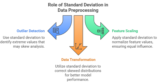
1. Outlier Detection: Identifying the Extremes

Outliers are values that significantly differ from the rest of your data. They can throw off ML models, especially those that rely on distance-based metrics like k-Nearest Neighbors (KNN) or Support Vector Machines (SVM). Standard deviation provides a simple yet effective way to identify these outliers.

• How It Works: A common approach to outlier detection is flagging data points that lie more than ±2 or ±3 standard deviations away from the mean. In a normal distribution, about 95% of your data should fall within 2 standard deviations from the mean. Values outside this range could be considered outliers.

This method works best on near-normal distributions; for skewed or non-normal data, alternative methods like the Interquartile Range (IQR) or Median Absolute Deviation (MAD) are often preferred.

• When to Use It: Outlier detection is crucial during exploratory data analysis (EDA), especially when you’re working with data that includes extreme values or when you plan to use robust regression techniques.
• Example: If you're analyzing customer purchase data, an unusually high transaction amount might be an outlier. Detecting it early can prevent your model from incorrectly learning patterns based on those extreme values.
• Practical Outlier Detection Methods: In practice, outlier detection can be done using scipy.stats.zscore() in Python to identify extreme values, or through visualizations like boxplots. These methods help you filter out or investigate outliers before training your model.

2. Feature Scaling: Equalizing Influence Across Features

In many datasets, features differ in scale. For example, “age” may range from 1 to 100, while “income” is in thousands. Standard deviation helps normalize these differences so that no single feature dominates the model due to its range.

• How It Works: The process of Z-score normalization uses standard deviation to scale data. Each value is transformed by subtracting the mean and dividing by the standard deviation. This results in features with a mean of 0 and a standard deviation of 1.
• When to Use It: Feature scaling is a must when using algorithms that are sensitive to the magnitude of features, such as Logistic Regression, Support Vector Machines, and neural networks. It’s also essential when performing principal component analysis (PCA) for dimensionality reduction.
• Example: Imagine you have a dataset containing both “age” and “salary”. Without scaling, your model might weigh salary (which can range from ₹30K to ₹300K) much more heavily than age (typically 20–80). Standardizing these features ensures that each one contributes equally to the model.
• Alternative Approaches: For datasets with outliers or non-Gaussian distributions, consider using a RobustScaler. Standard deviation can be inflated by extreme values, which skews Z-score scaling and may distort feature scaling. In contrast, IQR-based methods scale data based on the median and interquartile range (IQR), effectively ignoring extreme tails. This makes them more robust and reliable for handling noisy or skewed datasets.

3. Data Transformation: Correcting Skewed Distributions

Many ML algorithms assume that your data is normally distributed. If your data is skewed, this can result in higher standard deviations and inaccurate model predictions. Standard deviation-based transformations can stabilize variance and make your data more symmetric.

• How It Works: Logarithmic and Box-Cox transformations reduce the impact of extreme values and compress long-tailed distributions. This creates more consistent data, helping the model generalize better.

For example, you can apply a log transformation using np.log1p(x) in Python, or use scipy.stats.boxcox() to perform a Box-Cox transformation.

• When to Use It: Data transformations are essential when working with skewed data, which is common in domains like finance, such as income or transaction amounts, or sensor readings, like temperature and pressure. They also help when applying models like linear regression or time series forecasting, which assume data normality.
• Example: For a fraud detection model, transaction amounts are often right-skewed. By applying a log transformation to the data, you can compress the distribution, ensuring that the model doesn’t focus too much on extreme values, like one high-value transaction.

Strengthen your expertise in standard deviation ML and other core statistical concepts with upGrad's Master’s in Artificial Intelligence and Machine Learning – IIITB Program. Build industry-relevant data analysis skills and position yourself for impactful career opportunities in technology and analytics.

Now let’s understand how standard deviation serves as a guiding metric throughout the modeling process.

Also Read: Machine Learning Basics: Key Concepts and Essential Elements Explained

Role of Standard Deviation in Building Machine Learning Models

Standard deviation in machine learning plays a vital role throughout the process, including understanding data, training models, and evaluating performance. Let’s examine how standard deviation ML affects model performance, training consistency, error analysis, and regularization.

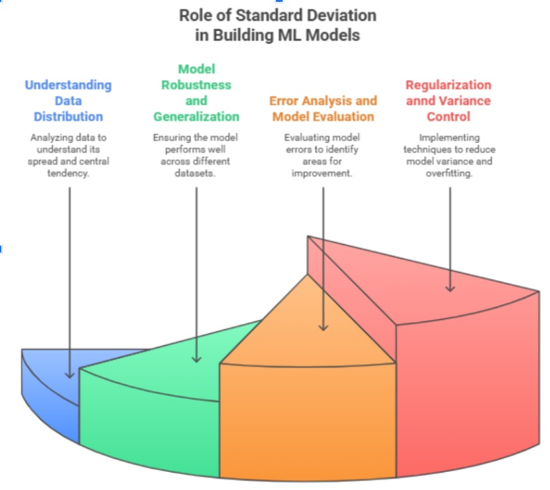
1. Understanding Data Distribution

Standard deviation quantifies the spread of data points around the mean. This helps you understand the variability of features in your dataset. Features with very different scales or high variance can negatively impact model training, especially for algorithms sensitive to scale (e.g., KNN, SVM, Neural Networks).

Code:

In this example, we are using NumPy to calculate mean and standard deviation for two sample groups.

import numpy as np
import matplotlib.pyplot as plt

# Sample data: heights (cm) of two groups
group1 = np.array([170, 172, 168, 165, 180])
group2 = np.array([160, 180, 150, 200, 170])

print("Mean group1:", np.mean(group1))
print("Std deviation group1:", np.std(group1))
print("Mean group2:", np.mean(group2))
print("Std deviation group2:", np.std(group2))

# Plotting
plt.hist(group1, alpha=0.5, label='Group 1')
plt.hist(group2, alpha=0.5, label='Group 2')
plt.legend()
plt.show()

Code Explanation:

• np.std() calculates the standard deviation of each group.

Output:

Mean group1: 171.0

Std deviation group1: 5.099

Mean group2: 172.0

Std deviation group2: 18.708

Output Explanation:

• Both groups have similar means (~171–172), but Group 2 has a much higher standard deviation (18.7), meaning its values are more spread out.
• This indicates higher variability in Group 2, which may impact model stability or performance.

Suggestion:

Use feature scaling, such as StandardScaler to standardize your features when working with algorithms sensitive to scale:

from sklearn.preprocessing import StandardScaler
import numpy as np
scaler = StandardScaler()
scaled_group2 = scaler.fit_transform(group2.reshape(-1,1))
print("Scaled Group 2 mean:", np.mean(scaled_group2))
print("Scaled Group 2 std deviation:", np.std(scaled_group2))

After scaling, the mean becomes 0 and the standard deviation becomes 1, making the data suitable for scale-sensitive models.

2. Model Robustness and Generalization

When using techniques like cross-validation, the standard deviation of performance scores reflects model robustness. A high standard deviation indicates inconsistent performance across data splits, suggesting overfitting or sensitivity to noise.

Code:

We use a Random Forest Classifier on the Iris dataset with 5-fold cross-validation. The accuracy scores across the folds are analyzed for standard deviation.

from sklearn.datasets import load_iris
from sklearn.model_selection import cross_val_score
from sklearn.ensemble import RandomForestClassifier
import numpy as np

data = load_iris()
X, y = data.data, data.target

model = RandomForestClassifier(random_state=42)
scores = cross_val_score(model, X, y, cv=5)

print("Cross-validation accuracy scores:", scores)
print("Mean accuracy:", scores.mean())
print("Standard deviation of accuracy:", scores.std())

Code Explanation:

• cross_val_score evaluates the model on five different data folds.
• scores.std() measures variability of the model's accuracy across folds.

Output:

Cross-validation accuracy scores: [1. 0.97 1. 0.93 1. ]

Mean accuracy: 0.98

Standard deviation of accuracy: 0.028

Output Explanation:

• The model achieves high accuracy across all folds.
• The low standard deviation (~0.028) indicates consistent performance and good generalization capability.

Suggestion: If you observe a high standard deviation:

• Simplify the model or use more robust techniques like Random Forest Algorithms or Gradient Boosting for stability.
• Perform stratified sampling during cross-validation to balance class distribution.

3. Error Analysis and Model Evaluation

The standard deviation of residuals (prediction errors) helps determine how consistently the model is predicting. A high residual standard deviation may signal poor fit or data/modeling issues. Ideally, the residuals should be centered around zero with minimal spread.

Code:

We train a Linear Regression model on the California housing dataset, predict test values, and calculate residuals (true - predicted). Then, we evaluate the mean squared error and standard deviation of residuals.

from sklearn.datasets import fetch_california_housing
from sklearn.linear_model import LinearRegression
from sklearn.model_selection import train_test_split
from sklearn.metrics import mean_squared_error
import numpy as np

# Load and split data
california = fetch_california_housing()
X_train, X_test, y_train, y_test = train_test_split(california.data, california.target, random_state=42)

# Train model
model = LinearRegression()
model.fit(X_train, y_train)
predictions = model.predict(X_test)

# Calculate residuals
residuals = y_test - predictions
print("Mean squared error:", mean_squared_error(y_test, predictions))
print("Std deviation of residuals:", np.std(residuals))

Code Explanation:

• After training a Linear Regression model, residuals are computed as the difference between actual and predicted values.
• np.std(residuals) shows the dispersion of prediction errors.

Output:

Mean squared error: 0.52

Std deviation of residuals: 0.71

Output Explanation:

• Mean squared error tells you how far, on average, your predictions are from the actual values.
• The standard deviation of residuals (~0.71) shows the consistency of prediction errors. Lower values indicate better reliability.

Suggestion:

• Plot residuals to visually inspect patterns or heteroscedasticity.
• If residuals have high spread, consider Robust regression (e.g., Huber Regressor) or Feature engineering to capture complex patterns.

4. Regularization and Variance Control

Regularization helps prevent overfitting by penalizing large model weights. This reduces the variance of predictions, indirectly reducing standard deviation across model coefficients. Models like Lasso or Ridge regression are designed to balance bias and variance using a regularization parameter (alpha).

Code: This code shows how increasing Ridge’s alpha shrinks coefficient variability by plotting their standard deviation.

from sklearn.linear_model import Ridge
from sklearn.datasets import fetch_california_housing
from sklearn.model_selection import train_test_split
import matplotlib.pyplot as plt
import numpy as np

# Load dataset
california = fetch_california_housing()
X_train, X_test, y_train, y_test = train_test_split(california.data, california.target, random_state=42)

alphas = [0.01, 0.1, 1, 10, 100]
coefs_std = []

# Train Ridge regression for different alpha values
for alpha in alphas:
    ridge = Ridge(alpha=alpha)
    ridge.fit(X_train, y_train)
    coefs_std.append(np.std(ridge.coef_))

# Plot std deviation of coefficients vs alpha
plt.plot(alphas, coefs_std, marker='o')
plt.xscale('log')
plt.xlabel('Alpha (Regularization Strength)')
plt.ylabel('Std deviation of coefficients')
plt.title('Effect of Ridge Regularization on Coefficient Spread')
plt.grid(True)
plt.show()

# Print the standard deviations for each alpha
for a, s in zip(alphas, coefs_std):
    print(f"Alpha: {a:<5} => Coeff Std Dev: {s:.4f}")

Code Explanation:

• Ridge regression is tested with increasing regularization strength (alpha).
• The standard deviation of the coefficients is calculated and plotted.
• Log scale is used because alpha spans multiple orders of magnitude.

Output:

Alpha: 0.01 => Coeff Std Dev: 0.6304

Alpha: 0.1 => Coeff Std Dev: 0.6242

Alpha: 1 => Coeff Std Dev: 0.5705

Alpha: 10 => Coeff Std Dev: 0.3130

Alpha: 100 => Coeff Std Dev: 0.0815

Output Explanation:

• As alpha increases, the standard deviation of the coefficients decreases.
• This shows regularization shrinks the coefficients and reduces model complexity, helping prevent overfitting.

If you observe large swings in model performance or very large coefficients, regularization with an optimal alpha can improve generalization and reduce overfitting risk.

Enhance your understanding of machine learning and advance your skills with upGrad’s Advanced Certificate Program in Generative AI. In just 5 months, gain hands-on expertise in generative models and position yourself for advanced roles in AI-driven innovation.

Let’s explore how standard deviation highlights performance consistency and helps you identify the most impactful features in your dataset.

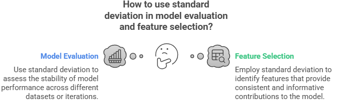
Utilizing Standard Deviation for Model Evaluation and Feature Selection

Standard deviation is important for assessing model performance and selecting relevant features. Here’s how it helps identify model stability and feature variability to improve results:

1. Model Evaluation: Measuring Performance Stability

In machine learning, hyperparameter tuning can cause variation in model performance across different training runs. Standard deviation ML helps quantify this variability, enabling you to identify hyperparameter settings that yield consistently strong results rather than just occasional high scores. This leads to more reliable and robust models.

• How It Works: When using k-fold cross-validation, you train and validate your model on multiple data splits. You typically get a set of performance scores such as accuracy, precision, recall, or F1-score. The standard deviation of these scores indicates how much your model’s performance varies across folds, reflecting its stability and robustness.
• When to Use It: Always check the standard deviation when comparing multiple models or tuning hyperparameters. A model with slightly lower accuracy but more stable performance may be more dependable in operational environments.
• Example: Imagine you’re developing a spam detection model. Two models might have similar accuracy, but if one shows a much higher standard deviation across validation folds, it may perform poorly on new, unseen data. In contrast, the more stable model is likely to generalize better.
• Tools That Show This: Platforms like scikit-learn, AutoML, and Google Vertex AI often include standard deviation metrics during evaluation. Make it a habit to review them alongside mean scores.

2. Feature Selection: Finding Informative and Stable Inputs

In a dataset, not all features are equally useful. Some vary meaningfully with the target variable, while others barely change or introduce noise. Standard deviation helps you filter out irrelevant or redundant features, improving model performance and training speed.

How It Works:

• Features with very low standard deviation have almost the same value for every record. These are often uninformative and can be dropped.
• Features with high but erratic variance might reflect outliers or measurement errors, and may need deeper analysis.

This technique is often a first-pass filter before more advanced feature selection methods like mutual information, recursive feature elimination (RFE), or SHapley Additive exPlanations (SHAP) values.

• When to Use It: Before applying heavy model training, use standard deviation ML to remove flat or static features. This is especially helpful in large datasets with hundreds or thousands of columns common in genomics, IoT, or Natural Language Processing pipelines.
• Example: In a health monitoring dataset with 500+ sensor readings, several features might show almost zero variation across patients. Removing these can dramatically reduce computational load without affecting model accuracy.
• Best Practice: Use standard deviation as part of a feature screening pipeline, but not the sole criterion. A feature might have low variance overall but still be predictive in certain subgroups; especially in imbalanced datasets.

Looking to strengthen your ML skills alongside standard deviation? upGrad’s Introduction to Natural Language Processing course provides essential NLP techniques such as tokenization, RegEx, and spam detection. Enroll today to develop practical skills that enhance your understanding of ML.

Also Read: Binomial Theorem: Mean, SD, Properties & Related Terms

Let’s see how standard deviation ML can fall short in challenging scenarios.

Challenges and Limitations of Standard Deviation in ML

While you often rely on standard deviation in machine learning models to understand data variability, it’s important to recognize its limitations. Being aware of these challenges will help you interpret this metric more accurately and avoid common pitfalls in your ML analysis.

Below are the key challenges to keep in mind when working with standard deviation iML.

1. Distribution Issues

Standard deviation can be misleading when data is skewed, multimodal, or contains outliers, as it is sensitive to extreme values and assumes a normal distribution. For example, in anomaly detection for right-skewed fraud datasets, applying standard deviation thresholds could miss fraudulent activities that lie outside of the expected range but still represent anomalies. In real-world applications like finance, healthcare, or user behavior modeling, these conditions often don't hold, leading to inaccurate thresholds and poor model performance.

Suggestion: Use robust alternatives like Median Absolute Deviation (MAD) or Interquartile Range (IQR) for non-normal data, and consider log or Box-Cox transformations to normalize the distribution before applying standard deviation-based methods.

2. Lack of Intuitive Understanding: Despite its statistical significance, standard deviation can be difficult to interpret, especially for business stakeholders or beginners. It may lack immediate interpretability, making it less useful for clearly communicating model insights. For instance, when presenting model results to non-technical stakeholders, a high standard deviation might be harder to explain compared to simpler metrics like ranges or percentiles which are more accessible.

Suggestion: Use visualizations (such as histograms or box plots), percentiles, or range-based summaries alongside standard deviation to improve clarity and foster better understanding of the data’s spread.

3. Inadequacy in Describing Complex Data Distributions: Standard deviation only measures the spread around the mean, ignoring the shape, skewness, or clustering of the distribution. In high-dimensional or non-linear datasets, this limitation can obscure important patterns, reducing the effectiveness of standard deviation in tasks like feature selection or model diagnostics. For example, in image classification or text modeling, where data is often sparse and complex, standard deviation alone won’t capture meaningful differences between classes or groups.

Suggestion: Use additional statistics like skewness and kurtosis, or apply advanced techniques such as clustering or dimensionality reduction (e.g., PCA) to better understand the underlying structure of the data.

Despite the challenges and limitations of standard deviation, it remains essential in many advanced ML methods. Let’s explore how it enhances important algorithms and statistical processes.

Beyond the Basics: Advanced Use of Standard Deviation

Advanced techniques require deeper statistical analysis and the integration of standard deviation into more complex ML workflows. Below, we explore its vital roles in dimensionality reduction, probabilistic modeling, statistical inference, and ensemble learning.

1. Use in Principal Component Analysis (PCA)

In PCA, standard deviation is related to variance, as PCA identifies the directions with the highest variance in the data. These directions (principal components) are used to reduce dimensionality, retaining the most important features while filtering out noise, which improves model performance in high-dimensional datasets.

2. Application in Gaussian-Based Models and Probabilistic Algorithms

In models assuming normality, such as Gaussian Naive Bayes or Gaussian Mixture Models, standard deviation ML defines the shape and spread of each distribution. Accurately estimating standard deviation is crucial for calculating likelihoods and posterior probabilities, directly impacting the model’s ability to classify or cluster data effectively.

3. Confidence Intervals and Statistical Tests

Standard deviation is fundamental for constructing confidence intervals around parameter estimates and model predictions. By quantifying variability, it allows practitioners to assess the statistical significance of results through hypothesis testing, ensuring that conclusions drawn from data are robust and reliable.

4. Variance Control in Ensemble Models (Random Forest, Bagging)

Ensemble methods like Random Forest reduce overfitting by averaging predictions from multiple decision trees. Monitoring the standard deviation ML of predictions across these trees provides insight into model variance and stability. A lower variance indicates more consistent predictions, which helps balance bias and variance for improved generalization.

In Random Forest, you can track prediction variance across estimators using methods like staged_predict or ensemble diagnostics, which allow you to observe how the predictions evolve across trees and identify any inconsistencies or areas for model tuning.

Looking to strengthen your data analysis skills for machine learning? upGrad’s Introduction to Data Analysis using Excel course provides comprehensive training in data cleaning, analysis, and visualization. Enroll today to develop essential skills and enhance your understanding of key concepts like standard deviation ML.

Advanced uses of standard deviation ML provide deeper insights into data variability, enhancing model performance and reliability in challenging scenarios.

How Well Have You Understood Standard Deviation ML?

Understanding standard deviation in machine learning models is key to building stable, reliable models. It helps evaluate performance consistency and identify meaningful features. Here are some questions that will let you assess how well you understand these core concepts.

1. What is the purpose of calculating standard deviation in machine learning models?

• To make the model more detailed
• To measure the variability or spread of data
• To reduce the dataset size
• To improve the speed of the model

2. Which of the following best describes standard deviation?

• The average of all data points
• A measure of data spread around the mean
• The highest value in the dataset
• The difference between minimum and maximum values

3. What is the first step in calculating standard deviation?

• Subtract the mean from each data point
• Calculate the variance
• Sum all data points
• Square the data points

4. How does standard deviation help in machine learning?

• By selecting features with the highest values
• By measuring how spread out the data is, aiding model performance
• By increasing dataset size
• By reducing the number of classes in classification

5. When calculating sample standard deviation, what divisor is used?

• N
• N - 1
• N + 1
• N / 2

6. Why might you normalize data using standard deviation?

• To reduce the number of samples
• To scale features to have a mean of 0 and standard deviation of 1
• To remove outliers completely
• To increase the dataset size

7. Which Python library is commonly used to calculate standard deviation?

• Matplotlib
• Numpy
• Pandas
• tensorflow

8. What does a high standard deviation indicate about the data?

• Data points are closely clustered around the mean
• Data points are widely spread out
• Data points are all equal
• Data points have no variation

9. How can standard deviation assist in anomaly detection?

• By identifying data points that fall far from the mean as potential outliers
• By increasing the dataset size
• By reducing data dimensions
• By improving computation speed

10. In which scenario is calculating standard deviation most useful?

• When all data points are identical
• When understanding the consistency or volatility of data is important
• When only the maximum value matters
• When working with categorical data only

Also Read: 15 Essential Advantages of Machine Learning for Businesses in 2025

Advance Your Skills in Standard Deviation ML with upGrad

Standard deviation ML is crucial for effective data preprocessing, model evaluation, and feature selection. By understanding the standard deviation formula and its application in machine learning, data scientists and ML engineers can improve model accuracy and make better data-driven decisions.

However, applying these statistical concepts with confidence in practical scenarios can be challenging. That’s where upGrad steps in, with expert-led programs in Data Science, Machine Learning, and Advanced Statistics that blend theory with hands-on training.

Here are some recommended courses to enhance your understanding of machine learning and help you excel in applying standard deviation ML and beyond.

• Generative AI Mastery Certificate for Data Analysis
• Generative AI Mastery Certificate for Managerial Excellence

Want to gain expertise in standard deviation ML in 2025? Reach out to upGrad for personalized counseling and expert guidance. You can also visit your nearest upGrad offline center to explore the right learning path for your goals.

FAQs

1. What is standard deviation, and why is it important in machine learning?

Standard deviation in machine learning models refers to how much data points vary from the mean, helping to measure data spread or variability. Think of it like volatility in stock prices, just as volatility shows how much stock prices fluctuate, standard deviation ML shows how much individual data points fluctuate around the average. In machine learning, understanding standard deviation ML helps assess data quality, guide preprocessing like scaling, and ensure the model isn't misled by unusual variations, improving its performance.

2. How does a high standard deviation affect a machine learning model's performance?

A high standard deviation indicates that data points vary significantly from the mean, much like high volatility in stocks where price swings can lead to unpredictable outcomes. In machine learning, this can cause a model to overfit, as it may try to capture random noise rather than meaningful patterns. Addressing high variability through normalization can help reduce this risk and improve model reliability.

3. What is the difference between variance and standard deviation in machine learning models?

Variance measures data spread by squaring deviations from the mean, while standard deviation ML is the square root of variance, bringing it back to the same units as the original data. For example, variance is like measuring how far volatility extends, but standard deviation is more intuitive, showing the actual spread of data points in the same terms as the data itself. This makes standard deviation easier to interpret when assessing variability in features for model development.

4. How can standard deviation be used to detect outliers in a dataset?

Just as a large market fluctuation indicates an outlier in stock prices, data points that fall more than 2 or 3 standard deviations from the mean are often considered outliers. Standard deviation in machine learning models helps identify these extreme values, which can skew results and hinder model performance. By flagging or removing outliers, you ensure the model learns more from the core patterns in the data.

5. How does feature scaling address high standard deviation in datasets?

Feature scaling, such as z-score normalization, uses standard deviation ML to adjust features, centering them around zero with a standard deviation of one. This is similar to comparing stocks in different currencies: by scaling features, you ensure each one contributes proportionally to the model, just as you'd normalize financial data across various markets. This avoids bias from features with higher variability, leading to better model training.

6. Why should we consider standard deviation when selecting features for machine learning models

When selecting features, understanding variability is crucial. Just as some stocks have higher volatility, features with extremely high or low standard deviation may carry too much noise or not provide meaningful distinctions. Standard deviation ML helps identify the features with meaningful variation, guiding the feature selection process and ensuring only the most relevant information is used in model training.

7. What is the impact of low standard deviation on a dataset in machine learning?

A low standard deviation means data points are tightly clustered around the mean, similar to a stock market with low volatility, where prices don’t fluctuate much. While this consistency can be useful, it may limit the model’s ability to capture complex relationships, potentially leading to underfitting. Standard deviation helps ensure there’s enough variation in the data for the model to learn effectively without missing key patterns.

8. How can standard deviation be used to assess the performance of a machine learning model?

Just as stock performance can be measured by price stability, the spread of performance metrics (like accuracy or error rates) across validation sets shows a model's consistency. A low standard deviation across multiple validation sets indicates stable performance, while a high standard deviation signals instability. This insight can help you adjust the model to be more reliable across different data subsets.

9. Why is it important to understand the statistical summary of the dataset in machine learning?

A statistical summary, including standard deviation, helps to understand the distribution and spread of the data. It's like reviewing the historical performance of a stock: by knowing how data is distributed, you can better detect anomalies, prepare for potential issues, and make more informed decisions in preprocessing and model design.

10. How can visualizing the correlation matrix help in understanding a dataset's structure?

A correlation matrix shows how features are related to one another. Pairing this with insights from standard deviation helps highlight how features vary and interact. For instance, if two highly correlated features both have high standard deviations, it could signal potential multicollinearity, just like noticing two volatile stocks that move in sync. Understanding these relationships helps refine feature selection and improves model design.

11. How do you calculate the standard deviation ML of a dataset in machine learning?

To calculate standard deviation ML, first find the mean of the data. Then, subtract the mean from each data point, square the results, find the average of those squared differences, and take the square root. Think of it like determining how much individual stock prices fluctuate around the average price in a given period—this helps you quantify data spread, guiding preprocessing and analysis decisions for model building.